Introduction
Mergers can have significant employment effects, potentially creating a trade-off between competition and jobs.Examples include proposed mergers between PSA and Fiat Chrysler (FCA), T-Mobile and Sprint, Albertsons and Kroger, or U.S. Steel and Nippon Steel. While competition authorities typically focus on consumer outcomes, employment impacts remain understudied and the explicit trade-off rarely evaluated.A nascent literature studies labor market power arising from overlaps in local labor markets (Prager and Schmitt 2021; Shapiro 2019; Marinescu and Hovenkamp 2019). By contrast, I examine employment effects absent such overlaps. This analysis is particularly relevant when firms face foreign competition, since blocking mergers might lead to aggregate employment losses.Many jurisdictions (e.g., Australia, China, France, Germany, Italy, Korea, the United Kingdom, South Africa) explicitly consider public interest in merger control ((OECD 2016)). While the European Union and the United States currently do not, worker interests have become increasingly prominent in merger control in these jurisdictions.
In this paper, I specify and estimate a structural model of demand and supply to study how foreign competition affects a merger’s consumer welfare and employment outcomes. I incorporate two key firm responses: price adjustments and product portfolio decisions. To capture the effects of product entry and exit on consumers and employment, I embed consumer demand into an endogenous product-choice model, where domestic labor demand depends on production locations and equilibrium product market quantities. My key methodological innovation is to construct a model that captures the interactions between the product market and labor demand. Using this framework, I estimate the average domestic job value at which employment gains offset consumer losses.
To illustrate this worker–consumer trade-off, I use the model to study the landmark Whirlpool–Maytag merger in the U.S. appliance market. I simulate consumer welfare and employment effects under two scenarios: the actual acquisition of Maytag by Whirlpool and a hypothetical acquisition by the alternative bidder at the time, the Chinese firm Haier. For tractability, production locations are treated as exogenous. In the Whirlpool scenario, I use observed post-merger locations; for Haier, I assume complete offshoring of Maytag’s production to China.This assumption follows anecdotal evidence about Haier’s bid, detailed in Section 2. Although an acquisition by Haier posed no direct threat to consumers (having no prior U.S. presence), its offshoring plans risked greater U.S. job losses.
Three main findings emerge. First, the Whirlpool acquisition is always worse for consumers. The merging parties increase prices without triggering significant rival product entry, causing an annual consumer welfare loss of $271 million. Second, Whirlpool preserves approximately 797 more U.S. jobs than Haier would have. Finally, each additional job preserved by Whirlpool (relative to a Haier acquisition) must be valued at about $344,000 annually to offset consumer losses.
While the worker–consumer trade-off in this application strongly depends on an alternative buyer’s offshoring plans, such a trade-off can arise more generally.For example, Stellantis CEO Carlos Tavares argued the FCA–PSA merger into Stellantis would improve competitiveness and prevent job losses ((Noble 2021)). Given sufficient information on counterfactual plant locations, the methodology outlined here can be applied to any merger or policy involving a worker–consumer trade-off.
The counterfactual simulations demonstrate that incorporating pricing and product assortment decisions significantly alters estimated employment effects, with important implications for studies of multinational enterprises (MNEs).For example, see Tintelnot (2017) or Arkolakis et al. (2023). Focusing on a single industry clarifies the trade-offs MNEs face in their global production decisions. In appliances, MNEs produce distinct product groups in different locations. Due to the oligopolistic market structure, cost changes at one location lead to adjustment of prices, product portfolios, and labor demand across locations for the affected firm and its rivals. This complements Muendler and Becker (2010), who analyze how employment at MNEs adjusts at both extensive (opening a new foreign location) and intensive margin (changing employment at an existing location) when different locations can complement or substitute each other’s production. While I focus only on intensive-margin adjustments, I explicitly model equilibrium effects following cost changes at particular locations. The results also complement Igami (2018), who studies the interplay between offshoring and market structure without employment implications.
For the empirical analysis, I assemble a comprehensive data set for U.S. residential laundry machines between 2005 and 2015. The core of the data comes from TraQline, a representative survey of 600,000 households per year. On the production side, I hand-collect product-level data on the locations of plants manufacturing for the U.S. market.
Using a difference-in-differences strategy similar to Ashenfelter et al. (2013), I document trends around Whirlpool’s acquisition of Maytag. Post-merger, U.S. market concentration rose significantly. Prices remained stable but fell in Europe, where Maytag was absent. Foreign rivals offered more products post-merger, but this was also the case in Europe. Finally, local unemployment increased following Maytag plant closures.
The descriptive evidence raises several questions. Was the expansion of rival product portfolios induced by the merger? Was consumer harm by the Whirlpool acquisition offset by benefits to U.S. workers? Answering these questions requires a model.
The model has two stages and features manufacturers and consumers. Manufacturers first choose product portfolios from technologically feasible options at fixed costs and hire workers.Since I observe only product-level entry but no firm-level entry around the time of the merger, I focus on endogenous product choices and abstract from firm entry. These decisions are based on expectations about second-stage sales and profits. Each product is associated with an exogenous set of characteristics, a production location, and a marginal cost of production. Whether a job is created domestically or abroad depends on the production location for each product. In the second stage, firms set prices, and consumers make purchases. Consumer demand follows a random coefficients discrete-choice model with income-dependent price sensitivity and heterogeneous tastes for front-loading washers, estimated following Berry et al. (2004). Identification exploits household-level income and price variation, second-choice characteristics, and an instrumental variable (IV) based on production locations and real exchange rates (RER), which is exogenous to product-level demand conditions (Goldberg and Verboven 2001; Grieco et al. 2024).
On the supply side, I estimate marginal costs assuming differentiated Bertrand-Nash competition. Fixed cost bounds for product offerings are estimated via moment inequalities, similar to Pakes et al. (2015) and methodologically closest to Eizenberg (2014). Intuitively, the fixed cost of offering a product that was offered can at most be the change in the expected variable profit due to the product. Similarly, the fixed cost of offering a product that is part of the set of potential products but was not offered must be at least as high as the change in variable profit due to the removal of that product.
I collect plant-level data to estimate the relationship between employment and output using a Leontief production function. I find that after a fixed employment threshold, output rises linearly with additional labor. Combined with the product-level plant locations, I can estimate how different product market equilibria affect the demand for domestic manufacturing workers. Furthermore,, I estimate how marginal costs vary with proxies for labor and transportation costs to compute how marginal costs react to changes in production locations.
Identifying the potential product sets for multiproduct firms is an empirical challenge.An earlier literature on endogenous product entry focuses on single-product firms with discrete product types (Mazzeo 2002; Seim 2006). I overcome this issue by exploiting an unconditionally cleared merger, where I observe the state of the world where the incentive for rivals to offer more products is greatest. Draganska et al. (2009) and Fan and Yang (2025) instead exploit cross-sectional variation. This is infeasible in my setting because portfolio decisions are national.
A second empirical challenge is equilibrium multiplicity for the counterfactual portfolio choice. Due to the large number of products, computing all potential equilibria is computationally infeasible. Instead, I follow a literature that uses heuristic learning algorithms to determine equilibrium portfolios (Lee and Pakes 2009; Wollmann 2018; Fan and Yang 2020). Each player optimizes her portfolio sequentially, taking the choices of rivals as given, until there is no profitable one-step deviation.
The simulation results indicate that each job preserved under an acquisition by Whirlpool (relative to Haier) would need to have an annual average value of at least $344,000 to offset the associated consumer harm ($238,000 if we consider the sum of consumer welfare and industry profits). By contrast, Flaaen et al. (2020) find that each job created by the 2018 washing machine tariffs was associated with an annual consumer harm of $800,000. Furthermore, Setzler and Tintelnot (2021) find an annual local wage bill gain of $113,000 per job created by foreign MNEs, excluding other employment benefits. Employment impacts are substantial and unevenly distributed. Whereas the losses to consumers are spread across the country, the employment effects are concentrated in a few local labor markets. While the gains from procompetitive competition enforcement likely outweigh losses, the results suggest that pairing it with complementary labor policies like wage insurance under the Trade Adjustment Assistance Program ((Hyman et al. 2023)) could increase its popular support.
Finally, I provide novel evidence that endogenous product portfolio decisions intensify consumer harm from mergers.Related work studies static entry for single-product firms (e.g., (Li et al. 2022), (Ciliberto et al. 2021)), dynamic multiproduct entry ((Garrido 2020)), post-merger repositioning ((Fan 2013)), and merger impacts on radio station variety (Berry and Waldfogel 2001; Sweeting 2010; Jeziorski 2015). Although product entry was key to the clearing decision for the Whirlpool–Maytag merger, I find that endogenous portfolio adjustments increase the harm to consumers. This is because the rival product portfolio expansion is mostly independent of the merger whereas the merging parties offer fewer products post-merger. Existing studies mostly consider hypothetical concentration changes and find mixed results.Fan and Yang (2020) find that endogenous product adjustments exacerbate negative consumer welfare effects, while Wollmann (2018) finds the opposite. Fan and Yang (2025) show that product portfolio adjustments exacerbate negative merger effects in small markets and reduce consumer harm in larger markets. Under certain conditions, Caradonna et al. (2025) show that without marginal cost efficiencies, product portfolio adjustments can only be profitable for the parties if there is harm to consumers.
The remainder is structured as follows: Section 2 describes the case and data, Section 3 provides descriptive evidence, Section 4 details the model, Section 5 describes estimation, Section 6 presents results, Section 7 describes welfare implications, and Section 8 concludes.
Institutional Setting and Data
In the mid-2000s, around 90 percent of washing machines sold in the U.S. were produced by the U.S. manufacturers Whirlpool, Maytag, and General Electric, which mostly produced domestically. While the Swedish Electrolux also manufactured in the U.S., LG and Samsung entered the market from plants in Mexico and South Korea.
Whirlpool’s acquisition of Maytag
Before its acquisition by Whirlpool, Maytag struggled financially despite workforce reductions and reported a net loss in 2004 ((Maytag 2005)). In May 2005, it initially agreed to a private investor buyout for $1.1 billion ((Barboza 2005)). Haier, a Chinese manufacturer, made a competing $1.3 billion bid in June 2005, but Whirlpool outbid it in July 2005 with $1.4 billion. On March 31 2006, Whirlpool acquired Maytag after receiving an unconditional merger clearance from the Department of Justice (DoJ).
Haier’s bid aligned with China’s “Go Out Policy”, encouraging overseas acquisitions to obtain access to foreign markets, particularly in the European Union and the United States, for Chinese manufactured goods ((Goodman and White 2005)). Since Chinese acquirers were met with resistance, these acquisitions often targeted well-known brand names slipping into decline. Maytag, with declining performance but strong brands, suited this strategy. Haier aimed to offshore production to China, using Maytag’s distribution channels and brand reputation ((Goodman and White 2005)).
Whirlpool’s bid prevented a foreign takeover but raised competitive concerns. The DoJ’s investigation focused on residential washing machines and dryers.See Armington et al. (2006) for a case description from the perspective of the DoJ. The DoJ cleared the merger despite high concentration, expecting foreign entrants like LG and Samsung to prevent price increases ((Department of Justice 2006)). Baker and Shapiro (2008a) call this decision “[...] a highly visible instance of underenforcement”, and Baker and Shapiro (2008b) describe it as “fueling the perception that the Justice Department has adopted a very lax merger enforcement policy [...]”. They conclude that, in this case, the DoJ was willing to accept entry and expansion arguments in a highly concentrated merger case despite the fact that entrants had thus far achieved only relatively low market shares.
Data
To analyze the implications of the Maytag acquisition, I construct a comprehensive data set on the U.S. market for residential laundry products between 2005 and 2015.
Sales, products, and households
The main data source, TraQline, is an annual survey of 600,000 U.S. households on appliance purchases, capturing product characteristics, prices, second-choice brands, retailers, and household demographics for which I have data for 2005–2015. The data set is well known across the appliance industry and is used by retailers and brands in the industry as a source for market insights.The only other comparable source of data on volume and value sales in the appliance industry is a (now discontinued) retailer panel by the NPD Group, which is the basis of the analysis by Ashenfelter et al. (2013). The data include information for washers and dryers and for freestanding ranges. I aggregate responses nationally and annually.
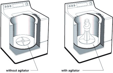
While TraQline records characteristics, respondents are not asked to provide the exact model specification. I therefore define a product as a brand, retailer, and key characteristic combination. Most brand owners use different brands to cluster their product offering according to the preferences of the consumers that they target.In its 2007 annual report, Whirlpool describes what each of its brands represents and what type of consumers it targets. Amana, for example, is described as stylish and affordable, whereas KitchenAid stands for quality and craftsmanship, Whirlpool for innovation and Maytag for reliability. Thus, the brand of a product already captures much of the variation in (otherwise unobserved) product differentiation. The key characteristic for washers is whether it is a regular top loader (with an agitator), a high-efficiency top loader (without an agitator) or a front loader. Finally, I refine the product definition by using information on the retailer at which the product is sold.For retailers, I distinguish Best Buy, H.H. Gregg, Home Depot, Lowe’s, Sears, and all others. The latter group predominantly includes smaller, regional retailers.
Households also need to report other characteristics of their purchases. For washers, these include child lockout features, the number of programs, or noise insulation. For each product, I calculate the average value of these characteristics among the subsample of respondents. I enrich these data with brand-level repair rates from Consumer Reports and advertising expenditures from Kantar AdSpender ((Benkard et al. 2021)).
I draw a random sample of households from the IPUMS Current Population Survey (CPS) to have data on the unconditional distribution of income in the population. I need this to identify how household income affects the sensitivity to prices in the demand estimation.
In the descriptive analysis, monthly data on model-level washing machine sales for Germany, France, Great Britain, and the Netherlands between 2005 and 2008 from Gesellschaft für Konsumforschung provide a control group for markets unaffected by the merger.
Production locations, cost shifters and employment
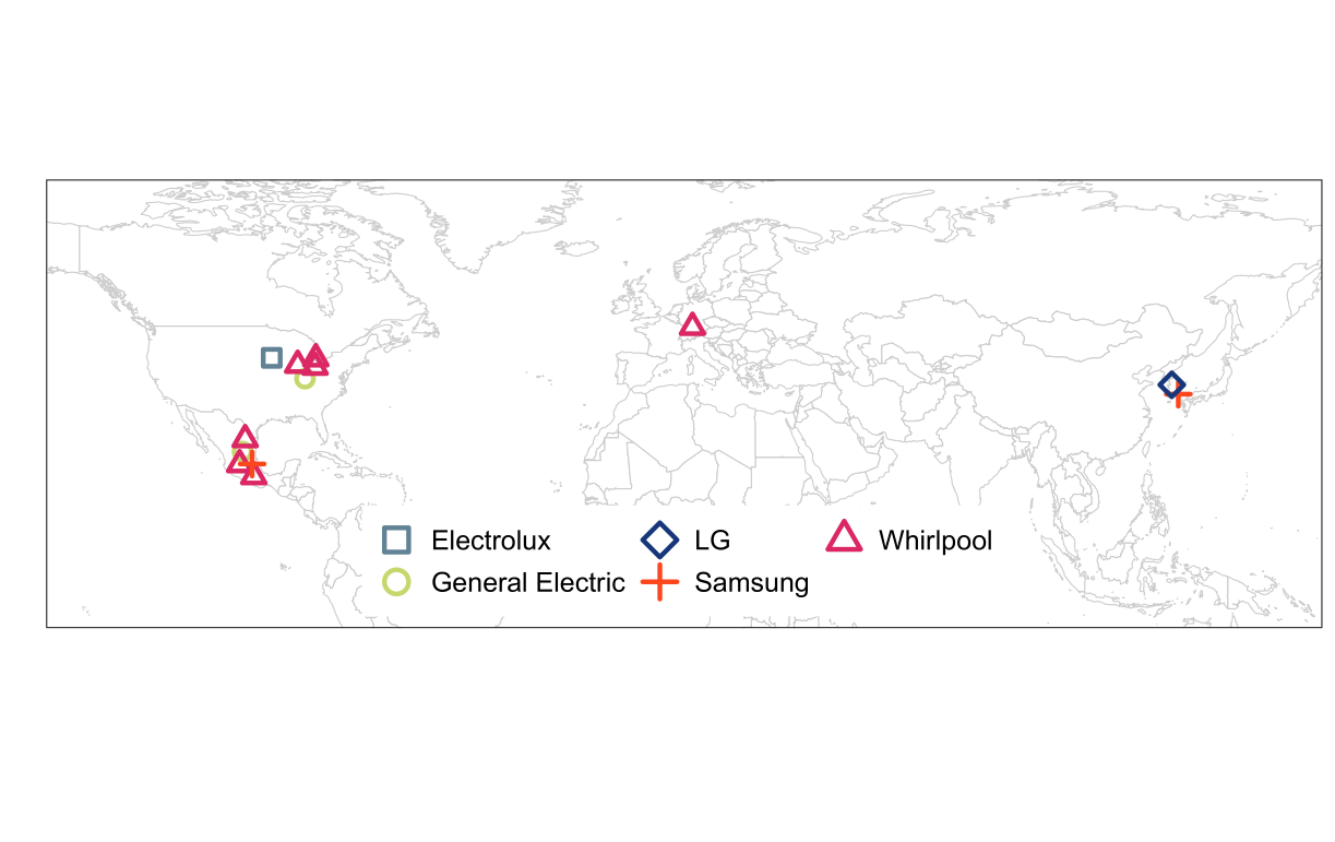
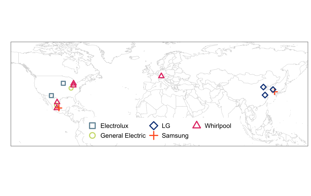
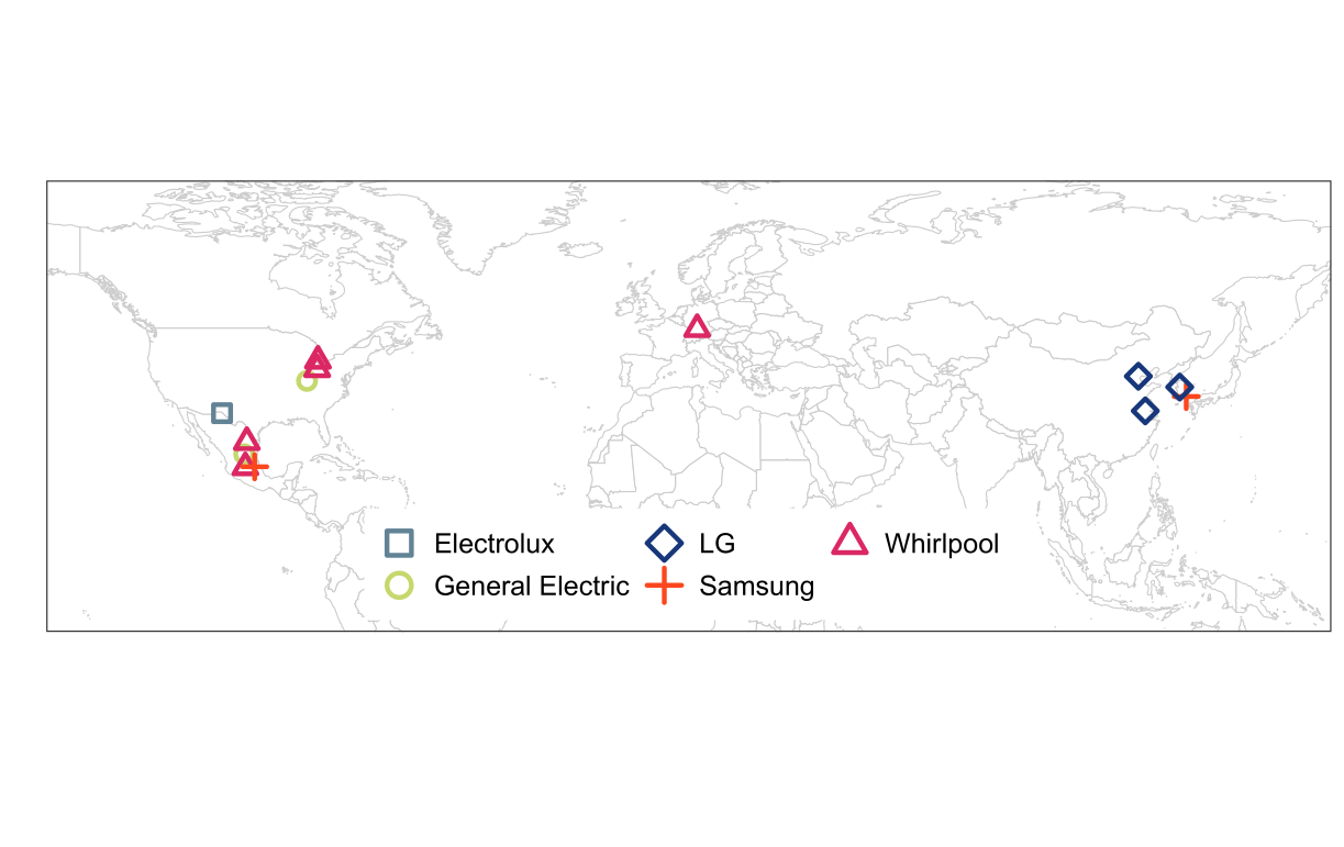
I hand-collect product-level manufacturing locations for washing machines for the U.S. market. Figure 1 shows the plant locations of major washing machine manufacturers in 2005. Details on the construction of this data set and the weights on the share of the products produced in each production location are described in Appendix 9.2.
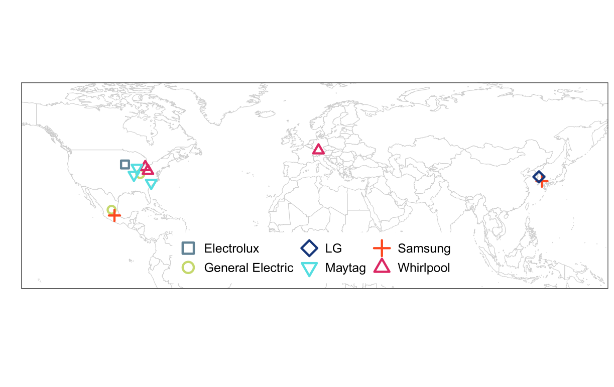
Pre-merger, Maytag production was entirely domestic, whereas Whirlpool’s top loaders were produced in the U.S. and most front loaders in Germany. Post-merger, Whirlpool restructured Maytag operations. Although it maintained some of Maytag’s manufacturing plants for other appliances (e.g. in Amana, Iowa, or Cleveland, Tennessee), it shut down laundry plants in Searcy, Arkansas (700 manufacturing jobs) and Herrin, Illinois (1,000 manufacturing jobs), as well as the laundry manufacturing and headquarter operations in Newton, Iowa (1,000 manufacturing and 1,800 corporate jobs).According to Maytag (2005), the company employed around 13,500 in its household appliance operations in the U.S. At the same time, Whirlpool announced adding a total of 1,500 jobs at an existing top loader plant in Clyde, Ohio and an existing dryer plant in Marion, Ohio. The production of Maytag front loaders, as well as new Whirlpool front loader models, moved to a production facility in Monterrey, Mexico.Moving Whirlpool front loader production to the Monterrey plant is not merger-specific, as Whirlpool announced eventually moving its front loader production for the U.S. to Monterrey in 2003 already.
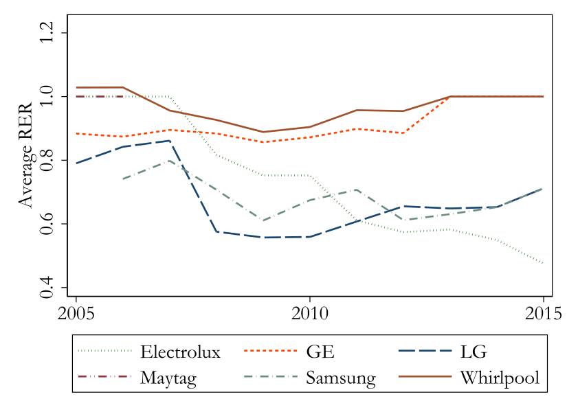
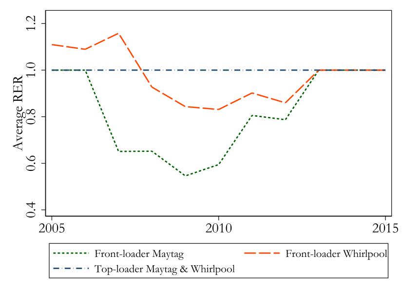
I construct a product-level cost shifter using the product-level weighted average real exchange rate between the U.S. and the countries in which the product is produced. The RER comes from the Penn World Table. Product-level plant weights are based on the share of a product produced in a particular origin country in a given year. I use the RER based on consumption expenditures. I calculate this by dividing the consumption of households at nominal prices by the the same consumption using the U.S. price level in 2005 and then multiplying this by the nominal exchange rate between the local currency and the U.S. dollar ((Feenstra et al. 2015)). The measure captures differences in relative price levels and serves as a proxy for local wage levels and nominal exchange rate fluctuations. Figure A.7 in Appendix 9.3 shows the evolution of the average RER over time and illustrates the source of the variation.
Estimating the relationship between plant-level output and employment requires plant-level data on both. Since these data are only sparsely available for plants producing for the U.S., I also consider BSH and Whirlpool plants that produce for the European market. In practice, the technology at a Whirlpool plant producing washing machines for the U.S. market in Germany appears to be similar to the technology at a Whirlpool plant producing washing machines for the European market. I collect data on annual plant output quantities and manufacturing workers employed between 1995 and 2017. In total, there are 25 plant–year combinations. Four of these belong to Whirlpool plants producing for the U.S. market, whereas 21 belong to BSH and Whirlpool plants producing for the European market. Details on the construction of this data set are described in Appendix 9.2.
Labor market data
To analyze the local labor market impacts of plant closures or employment increases at existing plants, I use wage and employment data from the Quarterly Census of Employment and Wages (QCEW) which includes quarterly county-level employment and compensation. I use the wages per employee and number of persons employed, disaggregated by county and industry. The wages include total compensation, bonuses, stock options, severance payments, the cash value of meals and lodging, tips, and other gratuities. I annualize these wages to ease interpretation. Unemployment data are drawn from Local Area Unemployment Statistics (LAUS). I construct matched control counties based on industry composition, demographics, and educational attainment. The industry composition is available annually in the QCEW, which I use for 2003 to 2006. The American Community Suvey (ACS) is not available at an annual frequency, which is why I use the 2005–2009 average as information on demographics and educational attainment from the 2009 ACS.
Descriptive Evidence
Before presenting the theoretical model, I describe concentration, prices, entry, and employment trends around the Maytag acquisition.
Changes in concentration
Table 1 shows brand owner market shares around the merger. Whirlpool and Maytag were previously the top domestic manufacturers, since Sears does not manufacture any appliances. Haier had no U.S. market presence.
The pre-merger Herfindahl–Hirschman index (HHI) and the post-merger increase indicate significant competitive concerns under U.S. merger guidelines.The HHI is calculated as the sum of squared market shares in whole percentages. According to the 2023 U.S. horizontal merger guidelines, markets with an HHI greater than 1,800 are considered highly concentrated. In such markets, an HHI increase of more than \(100\) is presumed to substantially lessen competition.
Notes: The table reports volume-based market shares by brand owner for washers and dryers pre-merger (2005) and post-merger (2007, 2009). The HHI is calculated as the sum of squared market shares in whole percentages. The increase in HHI is computed using pre-merger market shares.
Due to data limitations, I focus on washers from hereon after. Whereas I have access to detailed sales data for washing machine markets unaffected by the merger, I do not have comparable data for dryers. Similarly, I collect detailed information on the production locations of washers, whereas this is more difficult for dryers. On the product market side, the results can be expected to be similar. As shown in Table 1, market shares for washers and dryers evolve similarly. In Appendix 10, I show that some of the descriptive evidence for price effects and entry by LG and Samsung is similar for washers and dryers.
Evolution of prices
To assess merger-related price changes, I compare the logarithm of washer prices in the affected U.S. market to unaffected European markets.Ashenfelter et al. (2013) follow an alternative strategy by comparing prices to those of unaffected control products, incl. ranges. I replicate their analysis using the TraQline data in Appendix 10. In contrast to my results, they find no price effects of the merger for washers. I believe that relying on washer prices in unaffected market is a better control group because they are unaffected by the merger but are otherwise affected by similar demand and supply shocks. As Maytag had no significant presence in Europe, the latter serve as an appropriate control group subject to similar industry trends but unaffected by the merger.
I use quarterly data for the years 2005–2008 to estimate a separate event study for every country. Specifically, I estimate the parameters of the following model:
\[\begin{equation} \tag{1} ln(p_{it}) = \beta x_{it} + \delta_{b(i)} + \gamma_{t} + \epsilon_{it} \,, \label{eq: desc price} \end{equation}\] where \(i\) denotes a model of brand \(b\) at time \(t\), \(x_{it}\) are product characteristics, \(\delta_{b(i)}\) are brand fixed effects, \(\gamma_{t}\) are quarterly time fixed effects, and \(\epsilon_{it}\) are idiosyncratic product-level shocks. Product characteristics differ slightly by country, but generally include washer type and performance features. Standard errors are clustered at the model level.
A. Control group: Germany
B. Control group: France
C. Control group: Great Britain
D. Control group: Netherlands
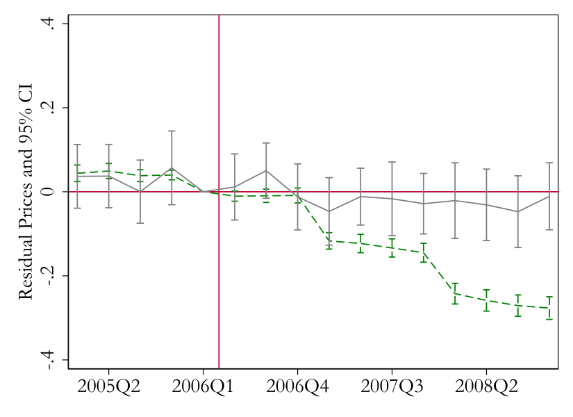
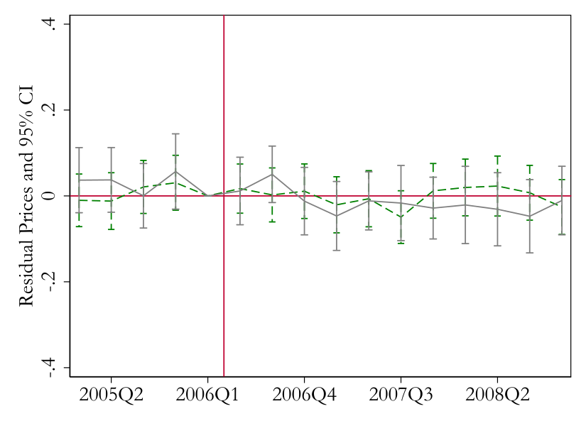
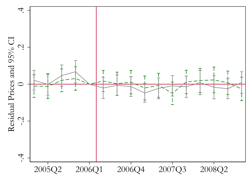
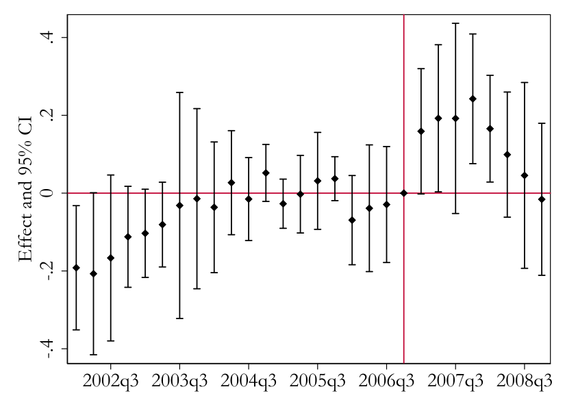
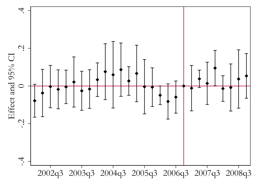
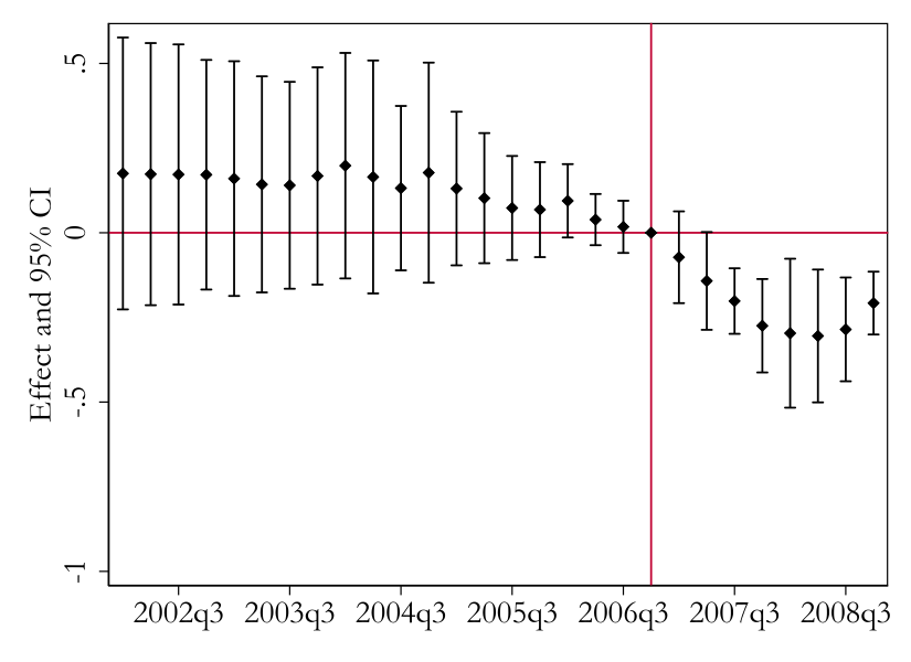
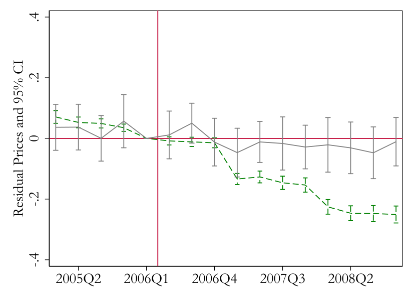
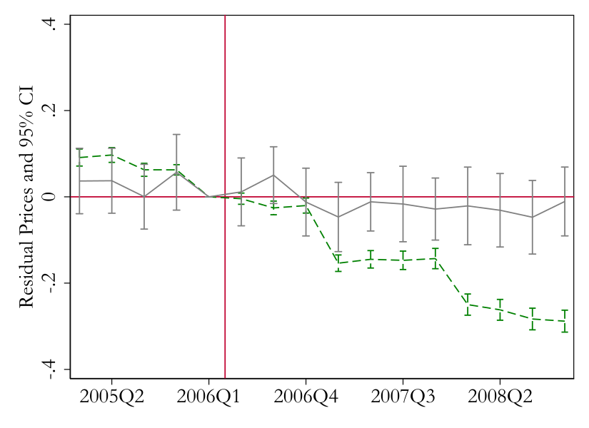
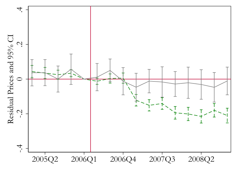
Notes: The figure displays the residualized log prices for Maytag and Whirlpool washing machines in the U.S. relative to washers from manufacturers in control countries unaffected by the merger. The merger occurred at the end of 2006Q1, normalized to zero. The solid line represents the U.S.; the dashed line represents the control group. Confidence intervals are at the 95% level, with standard errors clustered at the model level.
Figure 2 plots the residualized price evolution. Q1 of 2006, the quarter prior to which Whirlpool acquired Maytag, is normalized to zero. The merging parties reported that the integration process should take up to a year, which is why we should expect to see price effects of the merger from 2007 onwards.
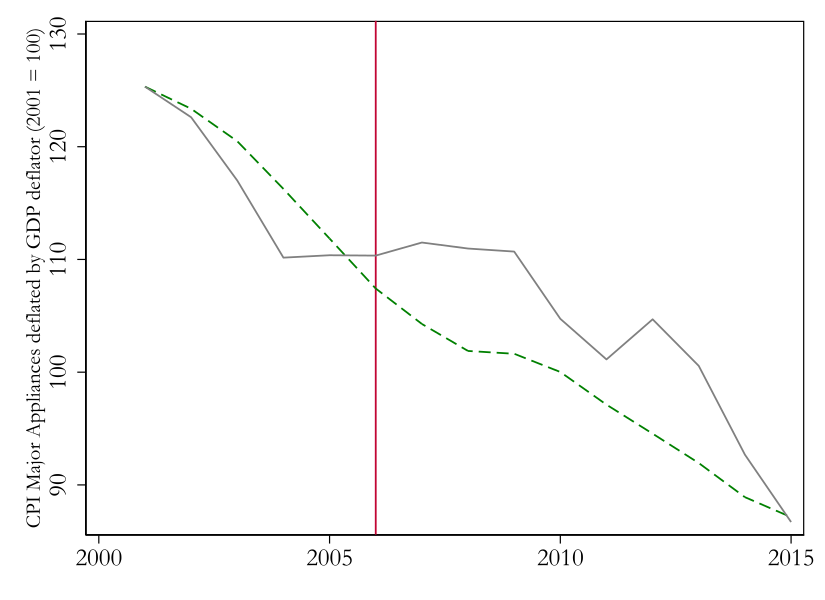
Prices in the U.S. and Europe tracked similarly pre-merger. Post-merger, European prices declined while U.S. prices remained stable. If the washing machine markets in the control countries are subject to similar industry trends on all aspects other than the merger, this suggests that the Maytag acquisition by Whirlpool significantly increased prices relative to their counterfactual evolution.In Appendix Figure A.9, I plot the evolution of deflated consumer price indices in the U.S. and EU between 2001 and 2015. The results corroborate the findings of the descriptive price analysis using GfK data.
Studying the price evolution in the U.S. without a control market, one might incorrectly conclude that the merger did not lead to price increases. However, this would miss cost decreases in the industry during the 2000s caused by a global trend to relocate production to low-cost countries. As shown in Figure A.7, most major manufacturers (including Whirlpool) relocated increasing shares of their production to lower-cost countries between 2007 and 2010.Appendix 9.3 documents quotes from the annual reports of, e.g., Electrolux and Maytag, to show that this was a key part of their business strategy at that time. Another explanation for price decreases in Europe is entry by new competitors from Asia (e.g., LG and Samsung), which occurred around the time of the merger.
Product entry
To assess the effects of the merger on consumers and workers, I need to understand whether rival product entry would have occurred even in the absence of the merger. Rival product entry could affect the estimated price effects of the merger in two distinct ways. First, if the merger led to merger-specific product entry, this could increase competition and decrease prices. Second, if there was merger-independent product entry by rivals around the time of the merger, this would also increase competition and reduce prices.
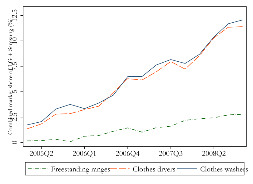
Figure 3 compares market shares of LG and Samsung in the U.S. versus several European markets. Both firms were active across all markets before the merger. Their combined share stagnated in Germany and Great Britain, while increasing in France, the Netherlands, and especially the U.S. This indicates that LG and Samsung’s U.S. expansion was likely not solely driven by the merger, though stronger U.S. growth raises the possibility of merger-induced entry.
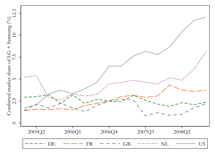
Notes: The figure shows the combined market share (volume sales) evolution in the U.S. and key European control markets from 2005 to 2008.
In Appendix 10, I document similar patterns for washers and dryers, highlighting minimal expansion by LG and Samsung in freestanding ranges, suggesting limited appropriateness of ranges as a control group.
Labor market effects of the acquisition
The analysis so far focused on the product market effects of the acquisition. Different acquisitions may also entail different changes to employment. For those to enter the overall welfare effects, appliance manufacturing jobs need to matter for local labor markets. In the following, I assess how the Maytag plant closures by Whirlpool post-acquisition affected employment, unemployment, and wages of the employed in the affected counties.
Although Whirlpool maintained some of Maytag’s manufacturing plants (e.g., in Amana, Iowa, and Cleveland, Tennessee), shortly after the acquisition, it shut down appliance manufacturing plants in Searcy, Arkansas (700 manufacturing jobs) and Herrin, Illinois (1,000 manufacturing jobs), and manufacturing and headquarters operations in Newton, Iowa (1,000 manufacturing and 1,800 corporate jobs). At the same time, Whirlpool announced the addition of 1,500 jobs at two existing plants in Ohio. There were thus three mass layoffs and two new job events. All of these were announced in 2006 and occurred in 2007.
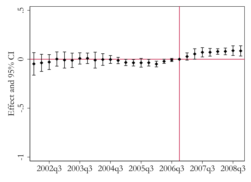
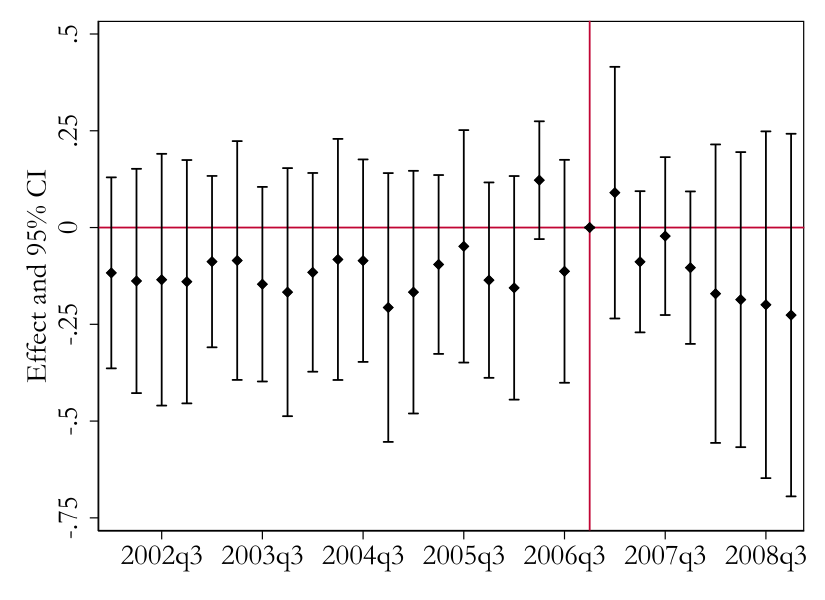
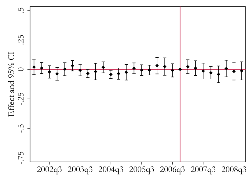
To quantitatively assess employment impacts from Maytag plant closures following Whirlpool’s acquisition, I use an event-study methodology inspired by Gathmann et al. (2020). I compare labor outcomes in treated counties to those in a set of matched control counties using an event study methodology.
I match a control group for every treated county that is similar on pre-treatment industry composition (21 different industries), as well as age structure (age groups 15–24, 25–49, and 50–66), education (low, medium, and high), and race (White, Black, and any other race). I do not match on any of the outcome variables of the employment analysis. Since I observe only a small number of events, I use the ten closest counties as a control group for every treated county instead of only the closest. Specifically, I calculate the normalized squared distance in the population share by characteristic of the treated counties to any other county in the United States.The distance equation for all treatment counties \(i\) and control counties \(j\) is given by \(distance_{ij} = \sum_{n} \omega_n \sum_{t} \frac{(x_{int} - x_{jnt})^2}{s_{nj}^2}\), where \(s_{nj}\) is the standard deviation of characteristic \(n\) in the control counties \(j\) and \(\omega_{n}\) is the weights of the different characteristics. Industry composition together has a weight of 50 percent, and each of the demographic characteristics accounts for a third of the rest. See Gathmann et al. (2020) for more details on the methodology. For the industry composition, I use annual data for the four years prior to treatment (i.e., 2003–2006), since annual county-level demographic characteristics are not available.
Next, I estimate the following event study:
\[\begin{equation} \tag{2} \text{Y}_{ct} = \sum_{\tau=2002}^{2006} \alpha_{\tau} \text{Event}_{ct}^{\tau} + \sum_{\tau=2007}^{2008} \beta_{\tau} \text{Event}_{ct}^{\tau} + \delta_{c} + \gamma_{t} + \epsilon_{ct} \,, \label{eq: desc jobs} \end{equation}\] where \(Y_{ct}\) is the logarithm of unemployment, manufacturing employment or annualized manufacturing wages in county \(c\) at time \(t\), \(\text{Event}_{ct}^{\tau}\) is an indicator equal to one if time \(t\) is in year \(\tau\) and county \(c\) is a treatment county, \(\delta_{c}\) is county fixed effects and \(\gamma_t\) is time fixed effects. Whereas data on unemployment are available at monthly level, the other outcome variables are available only at quarterly level. In each case, I use the most disaggregated level.
In the baseline specification, I use a simple difference-in-differences strategy, where I use data for 2002–2006 as the pre-treatment period and data for 2007 and 2008 as the post-treatment period.To avoid adding noise from the Great Recession, I do not use data for 2009. Appendix 10 includes graphical results for the full event study analysis, where there are separate quarterly treatment effects for the years prior to treatment (2002–2006) and the treatment years 2007 and 2008.
I group the counties into two different treatment groups and estimate separate regressions. The first treatment group consists of Jasper County, in which there was a shutdown of both manufacturing and corporate operations, as well as White and Williamson Counties, in which manufacturing plants were shut down. The second group consists of Marion and Sandusky Counties, where Whirlpool created new jobs.
| Unemployment | Employment | Wages | ||||||
| (1) | (2) | (3) | (4) | (5) | (6) | |||
| Mass layoff | 0.184\(^{***}\) | -0.348\(^{***}\) | -0.008 | |||||
| (0.058) | (0.123) | (0.048) | ||||||
| New jobs | 0.026 | 0.087\(^{***}\) | -0.004 | |||||
| (0.033) | (0.030) | (0.019) | ||||||
| County fixed effects | Yes | Yes | Yes | Yes | Yes | Yes | ||
| Time fixed effects | Yes | Yes | Yes | Yes | Yes | Yes | ||
| Observations | 2,520 | 1,596 | 840 | 532 | 840 | 532 | ||
Notes: The dependent variable is the logarithm of
county-level unemployment (Columns 1–2), manufacturing employment
(Columns 3–4), and manufacturing wages (Columns 5–6). Observations are
at the monthly level (Columns 1–2) or quarterly level (Columns 3–6).
Standard errors (in brackets) are clustered at the county level.
Significance levels: \(^{*}\) \(p<0.10\), \(^{**}\) \(p<0.05\), \(^{***}\) \(p<0.01\).
Table 2 reveals significant increases in unemployment (\(18\%\)) and decreases in manufacturing employment (\(35\%\)) due to closures. The increase in unemployment comes from a base of between 1,000 and 2,000 people per treated county. This is non-negligible, considering that it does not account for workers that are retraining and those that have temporarily or permanently left the workforce. The decrease in manufacturing employment is sizable and confirms the importance of the Maytag plants to local county employment. Each of the counties with Maytag plants employed between 3,000 and 4,000 workers in manufacturing. So this translates to a decrease in the number of workers equivalent to the Maytag job cuts.
Column (5) shows no significant effect on local average wages in manufacturing. Columns (2) and (4) show that although the newly created Whirlpool jobs did not affect local unemployment, they led to a statistically significant increase in local manufacturing employment. The results in Column (6) suggest that this did not affect average local manufacturing wages.
The event study plots in Figure A.11 confirm timing alignment with Maytag employment changes, underscoring the local significance of appliance manufacturing jobs. They also show that the treatment effects were still present in 2008, the second year after treatment. The results suggest that appliance manufacturing jobs matter for local labor markets and can have persistent effects on employment and unemployment. This conclusion is further supported by Gathmann et al. (2020), who show that mass layoffs also lead to sizable and persistent negative spillover effects to the local economy, and Jacobson et al. (1993), who show that high-tenure workers suffer long-term earnings losses after separating from distressed firms.
Model
Three observations emerge from the preceding analysis. First, product portfolio decisions played a key role in shaping product market outcomes, making them central to evaluating the merger effects. Second, while firms adjusted their product offerings, no new firm entered the market, allowing me to abstract from firm-level entry. Third, labor market frictions and differences in production locations imply that who produces where matters for welfare.
These observations inform a model with manufacturers and consumers. Manufacturers choose product portfolios and prices; consumers choose among available products. The model unfolds in two stages. In the first stage, firms are endowed with a set of potential products and associated production locations. They observe product-specific fixed cost shocks, choose which products to offer, and hire workers. At this stage, they do not observe transitory demand or marginal cost shocks and form expectations over them. In the second stage, these shocks are realized and observed. Firms set prices for the chosen products. Consumers then observe all product characteristics and make discrete purchase decisions. I solve the game backward by searching for the subgame perfect Nash equilibria (SPNE) of the game.Whenever cost or demand shocks are observed by market participants, they remain unobserved by the econometrician. To estimate the model parameters, I require the existence of a SPNE but not its uniqueness.
This framework captures the interaction between product market and labor market outcomes and provides a basis for evaluating the effects of different acquisitions.
Product portfolios
In the first stage, firms decide which products to offer and how to produce them. Each firm begins with a set of potential products \(\mathcal{J}_{ft}\) it can supply in market \(t\).Since I have only temporal variation, I use “market” and “time” interchangeably. This set comprises products already sold by the firm at different retailers or markets, and new variants resulting from minor modifications to existing products. It excludes products requiring entirely new technological capabilities (e.g., introducing a firm’s first front loader).Because the data do not distinguish between new and continuing products, I cannot estimate separate fixed-cost bounds for each type.
Offering a product involves a fixed cost, including final development, marketing, and retailer-specific investments. Empirically, I consider annual markets. Given that sales of specific appliance models decline rapidly within one year of launch ((Ashenfelter et al. 2013)), I assume the fixed cost of offering a product in a given year is independent of previous product portfolios.
The fixed cost \(F_{jt}\) of offering product \(j\) comprises a brand-specific component \(F_{b(j)}\) and a mean-zero product- and market-specific fixed-cost shock \(\upsilon_{jt}\), such that \(F_{jt}=F_{b(j)}+\upsilon_{jt}\), with \(E[\upsilon_{jt}|j\in\mathcal{J}_{ft}]=0\). Before portfolio selection, firms observe all product-specific fixed-cost shocks but not second-stage marginal cost and demand shocks, denoted \(e_{jt}=(\xi_{jt},\omega_{jt})\). Firms thus select their portfolios by balancing expected incremental variable profits for every product against the fixed costs of offering that product: \[\begin{equation} \displaystyle \max_{J_{ft} \subseteq \mathcal{J}_{ft}} \left\{ \pi_{ft} = E\left[VP(p) | J_{ft}\right] - \sum_{j \in J_{ft}} F_{jt} \right\} \,. \end{equation}\]
As portfolio selection is a discrete choice, optimality conditions hold only as inequalities.
Production and local labor demand
At the same time as firms choose their product portfolios, they also decide how to produce them. At this stage, firms form expectations about the second-stage shocks \(e_{jt}=(\xi_{jt},\omega_{jt})\), which are not yet realized or observed.
Each potential product is associated with fixed product characteristics and a production location. Because manufacturers typically produce a given washer model for the U.S. market at a single plant, knowing a product’s key characteristics allows me to identify its plant and thus its production country.
I model washer production using a Leontief technology: \[\begin{equation} \tag{3} \displaystyle q_{jt} = \min \left\{\lambda_{1f(j)} K_{jt}, \lambda_{2c(j)} L_{jt}, \lambda_{3j} M_{jt}\right\} \,, \label{eq: model prod} \end{equation}\]
where \(K_{jt}\), \(L_{jt}\), and \(M_{jt}\) are the amounts of capital, labor, and materials needed for producing quantity \(q_{jt}\) of product \(j\) at time \(t\). The marginal products \(\lambda_{1f(j)}\), \(\lambda_{2c(j)}\), and \(\lambda_{3j}\) correspond to capital, labor, and materials, respectively. Firms cannot substitute among inputs given these marginal products, but they may indirectly adjust marginal products through investments in technology or product selection. The marginal product of capital varies by firm (\(f(j)\)), labor by plant (\(c(j)\)) to capture scale economies, and material by product to accommodate differences between high- and low-end models.
Because employment effects of the merger are central to my analysis, the relationship between the number of workers and output is crucial. I assume each plant uses the same technology, differing only by size and potential economies of scale. Scale economies at the plant (rather than model) level seem appropriate, given that plants share many production processes across models and I observe employment and output data at the plant level. Table 8 confirms that most models are produced at a single plant.
I specify two potential relationships between plant-level output and employment. Appendix 11.1 specifies an alternative Cobb-Douglas production function, \(q_{c(j)t}=AL_{c(j)t}^{\zeta}\). I cannot reject \(\zeta=1\), indicating constant returns, but the fit to data is poor. Instead, Figure 4 plots annual plant-level output and employment for plants where this data is available. After splitting the sample according to the decade of the observation, the plot shows an approximately linear plant-level relationship between employment and output. This indicates that washer plants require a certain number of manufacturing workers to operate, after which output increases linearly in the number of workers. Although marginal costs appear to be constant, variable costs decrease with scale.
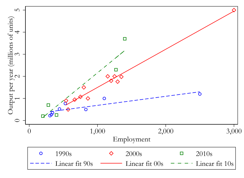
Notes: The figure shows the relationship between plant-level output and employment.
Furthermore, the slope of this relationship becomes steeper over time. This suggests that the marginal product of labor increases over time, most likely due to technological improvements. Overall, the data suggests that the marginal product of labor is constant between plants at a given point in time but increases over time. An important caveat here is that there is only limited data available on plant-level output and employment.
To formalize this, I specify the relationship as: \[\begin{equation} q_{c(j)t} = \begin{cases} 0 & \text{if } L_{c(j)t} < \psi_0, \\ \psi_1 \cdot (L_{c(j)t} - \psi_0) & \text{if } L_{c(j)t} \geq \psi_0, \end{cases} \end{equation}\]
where \(\psi_0\) is the overhead labor requirement for operating a plant without output, and \(\psi_1\) is the annual marginal product of labor. Estimating the inverse specification,
\[\begin{equation} L_{c(j)t} = \psi_0 + \psi_1^{-1} q_{c(j)t} + \rho_{c(j)t} \,, \end{equation}\]
where \(\rho_{c(j)t}\) captures measurement error in plant-level employment, yields the parameters in Table 3. Using the full sample, the overhead labor requirement \(\psi_0\) is 315 workers, dropping to 161 workers for observations from the 2000s. The estimated annual marginal product of labor, \(\psi_1\), is 2096 washers per worker for the full sample and 1780 washers per worker for the restricted sample, with a 95% confidence interval between 1585 and 2029.
| (1) | (2) | |
|---|---|---|
| \(\psi_0\) | 315.1516\(^{**}\) | 161.3267\(^{**}\) |
| [57.7550,572.5482] | [20.9060,301.7474] | |
| \(\psi_1^{-1}\) | 0.0005\(^{***}\) | 0.0006\(^{***}\) |
| [0.0003,0.0006] | [0.0005,0.0006] | |
| Restrict to 2000s | No | Yes |
| Observations | 25 | 12 |
Notes: The dependent variable is total plant-level
employment. Column (2) includes observations from 2000–2009 only. 95%
confidence intervals are shown in brackets. Significance levels: \(^{*}\) \(p<0.10\), \(^{**}\) \(p<0.05\), \(^{***}\) \(p<0.01\).
Marginal costs are additive due to the Leontief production technology. Including transportation, product-level marginal cost is: \[\begin{equation} \tag{4} \displaystyle mc_{jt} = \lambda_{1f(j)}^{-1} r_{f(j)t} + \psi_1^{-1} w_{c(j)t} + \lambda_{3j}^{-1} m_{t} + \tau_{t} d_{c(j)t} + \omega_{jt} \,, \label{eq: model mc} \end{equation}\] where \(r_{f(j)t}\), \(w_{c(j)t}\), and \(m_{t}\) are input prices for capital, labor, and materials; \(d_{c(j)t}\) is the distance between the production location of product \(j\) and the destination market; \(\tau_t\) is transportation cost per washer for every distance unit; and \(\omega_{jt}\) is a product-level marginal cost shock realized after input and portfolio choices. This can be thought of as an unanticipated shock to per-unit material costs.
Firms take input prices as given. Local labor market effects can arise even with competitive input markets. Suppose local labor markets have convex supply and worker mobility frictions, combined with fixed costs of operating a plant and sunk relocation costs. In this case, plant openings or closures shift local labor demand. Adjustments occur primarily via employment on the elastic portion of labor supply or via wages on the inelastic portion. While fully modeling local labor markets and estimating labor market power would allow more flexibility on the employment side, this is beyond the scope of this paper. Because Table 2 shows employment adjusted without wage changes following plant openings and closures, I assume labor markets operate on the elastic portion. Hence, I keep wages fixed and allow employment to adjust.
Even with efficient local labor markets, policymakers may choose to invest public funds to shift local labor demand (e.g., by offering tax incentives), provided the investment cost is lower than the resulting surplus. If manufacturers have wage-setting power, a merger-induced decrease in local labor demand could lower local wages, partially offsetting the employment loss (Kroft et al. 2025). However, since wages did not adjust in the descriptive analysis, this concern appears limited in this application.
Domestic labor demand for firm \(f\) can thus be expressed as: \[\begin{equation} LD_{ft} = \psi_0\times(\#\text{domestic plants}_{ft})+\sum_{j\in J_{ft}}\psi_1^{-1}E[q_{jt}]\times\text{domestic share}_{jt}, \end{equation}\] where \(\text{domestic share}_{jt}\) is the fraction of product \(j\) produced domestically.While most products are produced in a single plant, some transitional cases involve multiple plants. See Appendix Table 8. Firms choose employment based on expected equilibrium product market quantities, which depend indirectly on wages via marginal costs.
Pricing and product demand
In the second stage, firms observe demand and marginal cost shocks, then set prices. Each firm \(f\) chooses prices for its offered products, \(J_{ft}\), to maximize variable profits: \[\begin{equation} \tag{5} \displaystyle VP_{ft} = \sum_{j \in J_{ft}} (p_{jt} - mc_{jt}) s_{jt} S_t \,, \label{eq: vp} \end{equation}\] where \(p_{jt}\) and \(mc_{jt}\) are price and marginal cost of product \(j\) at time \(t\), \(s_{jt}\) is its market share, and \(S_t\) is total market size. Equilibrium prices satisfy the first-order conditions: \[\begin{equation} \tag{6} \displaystyle p_{jt} = mc_{jt} - [(\nabla_p s \bullet \Lambda)^{-1} s]_{jt} \,, \label{eq: foc} \end{equation}\] where \(\Lambda\) is the ownership matrix capturing firm-level product ownership, and \(\nabla_p s\) is the matrix of market-share derivatives with respect to prices.
Household demand for washers follows a discrete-choice framework as in Berry et al. (1995) and Berry et al. (2004). In each year, households either buy one washing machine from the available set \(J_t\) or choose an outside good (keeping their existing washer or having none).
Household \(i\)’s utility from washer \(j\) in year \(t\) is: \[\begin{equation} \tag{7} \displaystyle u_{ijt} = x_{jt} \beta + \sigma^{FL} \nu_{it}^{FL} x_{jt}^{FL} - exp(\alpha + \kappa_{\alpha} \iota_{it} ) p_{jt} + \xi_{jt} + \epsilon_{ijt} \,. \label{eq: utility} \end{equation}\] The vector \(x_{jt}\) includes non-price product characteristics (e.g., front loader indicator, brand repair rate, number of programs), brand and retailer dummies, year fixed effects, and brand-specific trends.Specifically, product characteristics include: brand repair rate, advertising expenditures, front loader, Korean front loader, Fisher & Paykel front loader, high-end European front loader (Asko, Bosch, Miele), agitator, stacked pair, stainless steel exterior, white exterior, Energy Star certification, extra noise insulation, child lockout, plus retailer, brand, and year fixed effects, and linear brand-specific trends. The price of washer \(j\) is \(p_{jt}\).
The average taste for non-price characteristics is captured by \(\beta\). Households differ in income \(\iota_{it}\) and in their idiosyncratic preference for front loaders \(\nu_{it}^{FL}\sim\mathcal{N}(0,1)\), scaled by \(\sigma^{FL}\). Price sensitivity varies exponentially with household income through parameters \(\alpha\) and \(\kappa_{\alpha}\), ensuring negative marginal utility of price.Household income is top-coded at $400,000. Although households with incomes above $400,000 are present in the household samples drawn from the CPS, TraQline groups all respondent households with an income above $250,000 together. In practice, setting a higher cap has negligible effects on estimated parameters.
The remaining utility components include a product-level unobservable common to all households, \(\xi_{jt}\), capturing unmeasured product quality and transitory demand shocks, and an idiosyncratic household-product shock, \(\epsilon_{ijt}\), drawn from a type-I extreme-value (Gumbel) distribution.
To simplify notation, I decompose utility into mean utility \(\delta_{jt}\) (constant across households) and household-specific deviations \(\mu_{ijt}+\epsilon_{ijt}\). Parameters of the demand model are collected in \(\theta=(\theta_1,\theta_2)\), with linear parameters \(\theta_1=(\beta)\) and nonlinear parameters \(\theta_2=(\sigma^{FL},\alpha,\kappa_{\alpha})\). The utility of the outside good is normalized to zero.
Given these distributional assumptions, market shares follow a familiar logit form. Integrating over the joint distribution of household demographics \(P_D(D)\) and taste shocks \(P_\nu(\nu)\) yields predicted market shares:
Connection between hiring and product market decisions
At first glance, product market and hiring decisions might seem only loosely connected. However, by explicitly modeling the link between output and employment and incorporating local production costs into product-level marginal costs, the model can capture how shifts in local production costs affect manufacturers’ labor demand.
For example, in 2005, Whirlpool produced most front loaders for the U.S. market in Germany, whereas Maytag produced them domestically. Both firms produced all top loaders domestically. Between 2005 and 2007, the German real exchange rate relative to the U.S. increased. Simultaneously, Whirlpool opened a front loader plant in Mexico post-merger while maintaining domestic top-loader production. Consequently, front loaders from Germany became relatively less attractive, and those relocated to Mexico more attractive. By 2009, Whirlpool had moved all front loader production for the U.S. market to Mexico. It then shifted it entirely back to the U.S. by 2013.
As local production costs for front loaders produced in Germany increased, but local production costs for front loaders relocated to Mexico fell, the share of German-made Whirlpool washers declined. The share of front loaders among Whirlpool’s post-merger sales rose from 24 percent in 2005 to 27 percent in 2007. When front loader production fully moved to Mexico, reaching its lowest relative cost compared to top-loaders, this share peaked at 29 percent. By 2013, after relocating front loader production entirely to the U.S., and hence increasing their relative production costs, front loaders accounted for only 19 percent of Whirlpool’s sales. Because labor demand is proportional to output, it increases when local production costs fall, and vice versa.
This is exactly what the model predicts. Given production locations, if production costs rise for some products but not others, firms reduce offerings of affected products and raise their prices, diverting sales toward products without a cost increase. This results in lower output and employment at plants facing higher local costs.
Estimation
This section describes the estimation of the model parameters, starting with demand, as later estimates build on these.
Demand
The demand estimation closely follows Berry et al. (2004). Full details on the moments and procedure are provided in Appendix 12.2; here I summarize how the data variation identifies the parameters.
As defined earlier, I partition the demand parameters \(\theta\) into linear parameters \(\theta_{1}\) and nonlinear parameters \(\theta_{2}=(\sigma^{\mathrm{FL}},\alpha,\kappa_{\alpha})\). I estimate \(\theta_{2}\) using the method of simulated moments (MSM) with three moment conditions. The first two moments match simulated household-level moments to their empirical counterparts, and the third exploits the orthogonality condition from excluding the real exchange rate cost shifter from utility. With three moments and three nonlinear parameters, the system is exactly identified. Conditional on \(\hat{\theta}_{2}\), the linear parameters \(\theta_{1}\) are estimated by ordinary least squares (OLS).
The first micro-moment matches the correlation between purchasing a front loader and the share of front loaders among second-choice brand for each household.See Equation (A.2) in Appendix 12.2. Although TraQline only records second-choice brands (not specific models), the front loader share differs considerably across brands. The correlation of \(0.4\) indicates unobserved taste heterogeneity for front loaders, influencing substitution patterns.
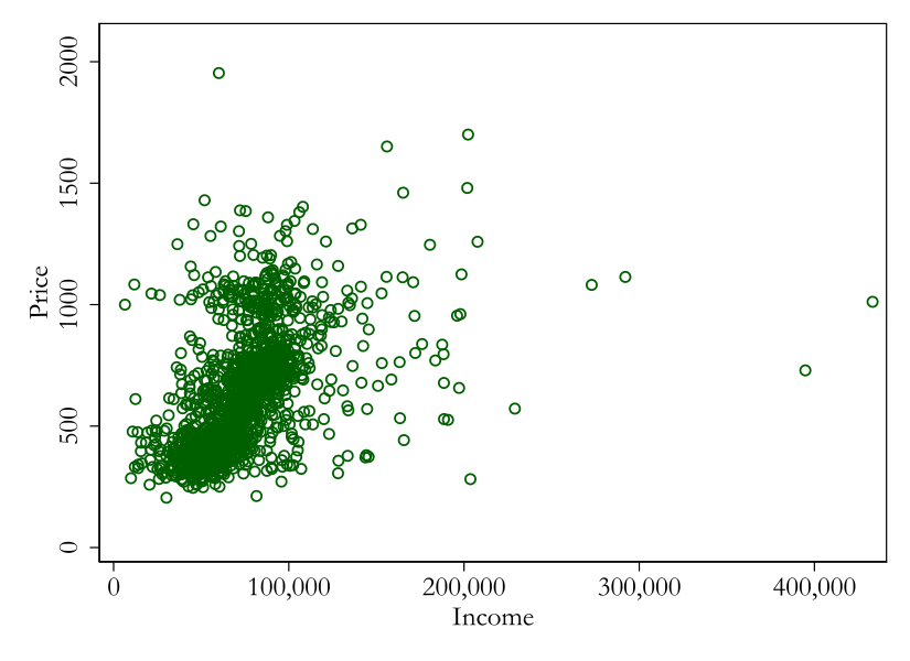
The second micro-moment matches the correlation between household income and washer purchase prices, which is \(0.5\).This corresponds to Equation [app eq: income mom] in Appendix 12.2. See also Figure A.12 for a scatter plot of the relationship between household income and price. This suggests lower price sensitivity among higher-income households.
To address price endogeneity due to correlation with the unobserved demand shock \(\xi_{jt}\), I instrument using the product-level real exchange rate described in Section 2. The RER captures product-level marginal cost variation from local wages and exchange rates at each production location but is orthogonal to U.S. product-level demand shocks, thus satisfying exogeneity. Both prices and the RER are deflated to 2012 dollars. For the specification with homogeneous price sensitivity, the RER is a conventional instrument; with heterogeneous price sensitivity, the nonlinear identification relies on the moment condition \(E[RER_{c(j)t}\xi_{jt}]=0\), preserving the exclusion restriction.
To estimate linear utility parameters \(\beta\), I first recover mean utilities \(\delta\) by matching simulated to observed market shares. For identification, I impose:
Assumption 1. \(E[e_{jt} | X_{jt}, F_{jt}] = 0\) for each \(j \in \mathcal{J}_{t}\).
Thus, second-stage demand and marginal cost shocks are independent of nonprice characteristics and fixed costs of offering a product. Following Eizenberg (2014), this assumption is slightly stronger than assuming \(e_{jt}\) is realized after product choices, as firms cannot predict these unobservable, transitory shocks. Nonetheless, firms may still predict demand and costs related to observables, which are controlled for explicitly.
An essential input for the demand estimation is market size, defined as the fraction of the population considering a washer purchase. TraQline provides total respondent counts, including non-buyers. Given washers’ roughly ten-year lifespan and the fact that households may start considering purchasing a new washer in the years prior to the end of a washer’s lifespan, I assume every seventh household considers buying a washer annually, making market size one-seventh of the surveyed households each year.
Standard errors for all demand parameters are clustered at the brand level using a residual bootstrap.
Marginal costs and production
I compute marginal costs by inverting each firm’s first-order conditions for profit maximization. Under the stated assumptions, each product has a unique marginal cost and markup that rationalizes the data.
The decomposition of marginal costs follows directly from Equation (4). I estimate: \[\begin{equation} \tag{9} \displaystyle mc_{jt} = FE_f + \gamma_1 RER_{c(j)t} + \gamma_2 d_{c(j)t} + \gamma_3 x_{j} + \omega_{jt} \,. \label{eq: estimation mc} \end{equation}\]
Firm fixed effects \(FE_f\) capture differences in capital intensity across firms. The real exchange rate \(RER_{c(j)t}\) is a product-level cost shifter capturing local wage and nominal exchange rate fluctuations. Given constant returns to scale, marginal costs scale linearly with wages, implying \(\gamma_1\) absorbs the labor productivity parameter \(\psi_1^{-1}\) from Equation (4). Distance \(d_{c(j)t}\) measures distance from each plant to the market center. The vector of nonprice characteristics \(x_j\) captures material cost differences across products, while \(\omega_{jt}\) denotes transitory material cost shocks. Finally, the estimated residual \(\widehat{\omega}_{jt}\) is computed as the difference between observed and predicted marginal costs.
Fixed cost bounds
The product assortment model in Section 4.1 yields inequality conditions, precluding point identification of fixed costs. Instead, I use partial identification to estimate bounds on these fixed costs for each brand.
To obtain fixed-cost bounds, I first define each firm’s set of potential products. This includes all products the firm could have offered (potential products, denoted \(\mathcal{J}_{ft}\)), distinguishing between those actually offered (active products, denoted \(J_{ft}\)) and those not offered (inactive products, denoted \(\tilde{J}_{ft}\)).
The set of potential products includes all products a firm is technologically capable of producing. The active products are observed in the data. I identify inactive products as variations of active products that the firm did not offer. For any active product (e.g., a front loader by KitchenAid sold at Sears), all versions of the product that I do not observe in the data (e.g., a front loader by KitchenAid sold at another retailer) is an inactive product. Thus, if a firm does not offer any front loaders, I do not assume it could have introduced one in that year. The fixed costs thus reflect marketing expenditures, retailer-specific investments, and product customization, but exclude costs of developing entirely new technologies.
I follow the procedure in Eizenberg (2014) closely to estimate these bounds. Under the assumption that observed product entry corresponds to a pure-strategy subgame-perfect Nash equilibrium, no firm can unilaterally deviate profitably. In practice, I estimate fixed-cost bounds using conditions derived from the absence of profitable one-step deviations.Additional restrictions could come from multi-step deviations. However, idiosyncratic fixed-cost shocks \(\upsilon_{jt}\) for different products make these difficult to incorporate.
I denote the equilibrium product portfolio (i.e., the set of active products) of firm \(f\) at time \(t\) as \(J_{ft}^{\ast}\). For each active product \(j\), the fixed cost is bounded above by the expected incremental profit from offering that product, holding other products fixed: \[\begin{equation} \displaystyle F_{jt} \leq E[VP_{ft}(J_{ft}^{\ast}) - VP_{ft}(J_{ft}^{\ast} - \mathbf{1}_{ft}^j)] \equiv \bar{F}_{jt} \,, \end{equation}\] where \(\bar{F}_{jt}\) is the upper bound on the fixed costs of offering product \(j\) at time \(t\).
Similarly, for each inactive product, the fixed cost is bounded below by the expected incremental variable profit if the product were added, again holding other products fixed: \[\begin{equation} \displaystyle F_{jt} \geq E[VP_{ft}(J_{ft}^{\ast} + \mathbf{1}_{ft}^j) - VP_{ft}(J_{ft}^{\ast})] \equiv \underline{F}_{jt} \,, \end{equation}\] where \(\underline{F}_{jt}\) is the lower bound on the fixed costs of offering product \(j\) at time \(t\).
Directly estimating the upper bound using active products and the lower bound using inactive products would be inadmissible since product portfolio decisions depend on \(\upsilon_{jt}\). However, the product-specific fixed cost shocks have mean zero conditional on the product being part of the set of potential products. With estimates of the lower bound of fixed costs of offering active products and estimates of the upper bound of fixed costs of offering inactive products, I can thus construct unbiased bounds on brand-level average fixed costs \(F_{b(j)}\).
Assumption 2. \(\sup_{j \in \mathcal{J}_{bt}} {F_{jt}} = F_{b(j)t}^{U} < \infty\) and \(\inf_{j \in \mathcal{J}_{bt}} {F_{jt}} = F_{b(j)t}^{L} > - \infty\) (bounded support)
Assumption 2 requires bounded support for fixed costs. While unlimited costs may be plausible for breakthrough technologies, here fixed costs reflect the costs of offering a product at another retailer or incremental product adjustments within existing technological capabilities. Thus, an upper bound seems plausible. Since costs of product introduction are always nonnegative, a finite lower bound \(F_{b(j)t}^{L}\) is also natural.
Assumption 3. \([F_{b(j)}^{L},F_{b(j)}^{U}]\subseteq\mathrm{supp}(\)expected incremental profit from adding or removing any single product of brand \(b)\)
Assumption 3 further restricts the fixed-cost support. Specifically, the fixed-cost distribution for potential products of brand \(b\) must lie within the range of expected incremental variable profits from adding or removing any single brand-\(b\) product. The intuition is straightforward: If a brand includes a blockbuster product so profitable that it is always offered, then this product is always part of the set of active products. Thus, the incremental variable profit of the most profitable product among the active products sets an upper bound on all fixed costs. Similarly, if there exists a potential product that is so unprofitable such that it is never offered, then its incremental variable profit sets a lower bound for fixed costs.
I fill in the missing lower bounds for active products using the minimum expected incremental variable profit among inactive products of the same brand. Conversely, missing upper bounds for inactive products are assigned using the maximum incremental variable profit among active products of that brand. Thus, product-level bounds on fixed costs for active and inactive products become:
2
\[\begin{equation} L_{jt}(\theta) = \begin{cases} V^{L}_{b(j)t}(\theta) & j \in J_{bt} \\ \underline{F}_{jt}(\theta) & j \in \tilde{J}_{bt} \end{cases} \notag \end{equation}\]
\[\begin{equation} U_{jt}(\theta) = \begin{cases} \bar{F}_{jt}(\theta) & j \in J_{bt} \\ V^{U}_{b(j)t}(\theta) & j \in \tilde{J}_{bt} \end{cases} \notag \,. \end{equation}\]
Since \(E[\upsilon_{jt} | j \in \mathcal{J}_{ft}] = 0\), and with the estimates of the upper and lower bounds on fixed costs for all \(j \in \mathcal{J}_{ft}\), applying unconditional expectations yields unbiased bounds on brand-level fixed costs: \[\begin{equation} \tag{10} E[L_{jt}(\theta)] \leq F_{b(j)t} \leq E[U_{jt}(\theta)] \quad \forall j \in \mathcal{J}_{bt} \,. \label{eq: identif fc set} \end{equation}\]
Next, I estimate the components of Equation (10). In Section 7, I analyze how the merger affects the incentives of brand owners to adjust their product portfolios using product portfolios in 2005 (pre-merger) and 2007 (post-merger). I therefore use the same two years’ data to estimate fixed-cost bounds.
For inactive products, I replace the population parameter \(\theta\) with its estimator \(\hat{\theta}\), yielding \(L_{jt}(\hat{\theta})=\underline{F}_{jt}(\hat{\theta})\) for \(j\in\tilde{J}_{bt}\). Similarly, for active products, \(U_{jt}(\hat{\theta})=\bar{F}_{jt}(\hat{\theta})\) for \(j\in J_{bt}\). Expectations are approximated using the sample mean across 500 draws from the joint empirical distribution of the demand and marginal cost shocks, \(e_{jt}\). Then, I use \(\min_{j \in \tilde{J}_{bt}}\{\underline{F}_{jt}(\hat{\theta})\}\) as an estimator for \(V^{L}_{b(j)t}(\theta)\) and \(\max_{j \in J_{bt}}\{\bar{F}_{jt}(\hat{\theta})\}\) as an estimator for \(V^{U}_{b(j)t}(\theta)\).
The resulting estimated interval for each brand is given by: \[\begin{equation} \left[\bar{l}_{n}^{b}(\hat{\theta}),\,\bar{u}_{n}^{b}(\hat{\theta})\right],\quad\text{where}\quad\bar{l}_{n}^{b}(\hat{\theta})=\frac{1}{n^{b}}\sum_{j=1}^{n^{b}}L_{j}(\hat{\theta}),\quad\bar{u}_{n}^{b}(\hat{\theta})=\frac{1}{n^{b}}\sum_{j=1}^{n^{b}}U_{j}(\hat{\theta}), \end{equation}\] and \(n^{b}\) is the number of potential products for brand \(b\). This procedure yields unbiased and conservative fixed-cost bounds.
Finally, I construct \((1-\alpha)\times 100\%\) confidence intervals for \(F_{b}\) following Imbens and Manski (2004) and Eizenberg (2014). These intervals are based on one-sided bounds around the point estimates: \[\begin{equation} \left[\bar{l}_{n}^{b}(\hat{\theta})-\frac{S_{l}(\hat{\theta})}{\sqrt{n^{b}}}z_{1-\alpha},\quad\bar{u}_{n}^{b}(\hat{\theta})+\frac{S_{u}(\hat{\theta})}{\sqrt{n^{b}}}z_{1-\alpha}\right], \end{equation}\] where \(S_{l}(\hat{\theta})\) and \(S_{u}(\hat{\theta})\) are standard deviation estimators for \(L_j\) and \(U_j\). I obtain these estimates using 200 bootstrap samples, which also account for variability in demand parameter estimates and variable profit simulations.
Parameter Estimates
Demand
Table 4 presents the demand estimates. Column (1) reports the first-stage regression, relating washer prices to the real exchange rate instrument, controlling for all covariates and fixed effects. A one-unit increase in RER raises prices by $203. The Kleibergen–Paap F-statistic of 31 indicates a strong instrument.
| (1) | (2) | (3) | (4) | |
|---|---|---|---|---|
| First stage | Logit OLS | Logit IV | Mixed logit | |
| Dependent variable: | Price | \(\hat{\delta}_{jt}\) | \(\hat{\delta}_{jt}\) | |
| Linear parameters | ||||
| Real exchange rate | 2.033\(^{***}\) | |||
| (0.365) | ||||
| Price (’00 2012 $) | -0.164\(^{**}\) | -0.351\(^{**}\) | ||
| (0.062) | (0.178) | |||
| Nonlinear parameters | ||||
| Common price coefficient \(\alpha\) | -0.676\(^{***}\) | |||
| (0.033) | ||||
| Income effect \(\kappa_{\alpha}\) | -0.209\(^{***}\) | |||
| (0.024) | ||||
| Unobserved taste \(\sigma^{FL}\) | 2.493\(^{***}\) | |||
| (0.068) | ||||
| Characteristics | Yes | Yes | Yes | Yes |
| Retailer FE | Yes | Yes | Yes | Yes |
| Brand FE | Yes | Yes | Yes | Yes |
| Brand time trends | Yes | Yes | Yes | Yes |
| Year FE | Yes | Yes | Yes | Yes |
| Observations | 1,590 | 1,586 | 1,590 | 1,590 |
| Kleibergen–Paap F-statistic | 31.041 | |||
| Avg. own-price elasticity | -0.964 | -2.058 | -2.542 |
Notes: Column (1) reports the first-stage regression results of prices on the real exchange rate. Column (2) presents estimates from the simple logit model without instrumentation. Column (3) shows estimates from the simple logit using the RER as an instrument for price. Column (4) displays results from the mixed logit model described in Section 4. Standard errors are clustered at the brand level. Own-price elasticities of residual demand are computed at the product level and averaged across products, weighting by sales volume. Estimates for nonprice characteristics are presented in Table 11. Significance levels: \(^{*}\) \(p<0.10\), \(^{**}\) \(p<0.05\), \(^{***}\) \(p<0.01\).
The remaining columns use the estimated mean utility of purchasing product \(j\) at time \(t\), \(\delta_{jt}\), as the dependent variable. Columns (2) and (3) report estimates from the simple logit model, first by OLS, then by IV. Accounting for price endogeneity decreases the average own-price elasticity from \(-0.96\) (OLS) to \(-2.06\) (IV). Column (4) shows the nonlinear parameters from the full mixed-logit model. These estimates highlight significant household-level heterogeneity in preferences. Higher-income households exhibit lower price sensitivity. Moreover, households purchasing front-loaders have systematically higher unobserved preferences for front-loaders. Incorporating these heterogeneities, the average own-price elasticity further decreases to \(-2.54\).
Marginal cost and production
Figure 5 displays the distribution of estimated marginal costs across all products.
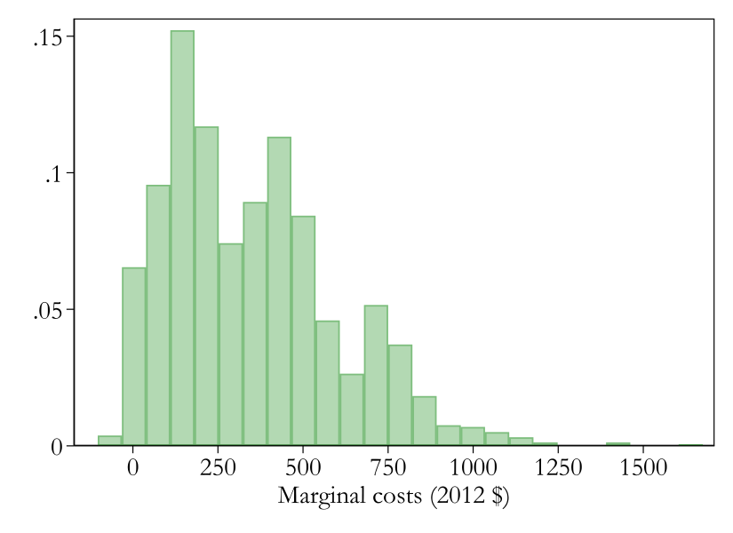
Notes: Histogram of estimated marginal costs (deflated to 2012 dollars) across all products in the sample.
Figure 6 plots marginal costs and Lerner indices by brand owner over time. Although marginal costs decline around the merger, this decrease occurs industry-wide, affecting both merging parties and rival firms. Hence, these cost reductions are not merger-specific, and any counterfactual analyses must reflect this broader trend. The observed cost pattern aligns with the decline in European washer prices documented in Section 3 and is consistent with general industry-wide savings through production relocation and technological advances. Concurrently, markups—as captured by Lerner indices—increase.The pronounced fluctuation in Samsung’s Lerner index between 2006 and 2007 should be interpreted cautiously, due to the small number of Samsung products available at that time.
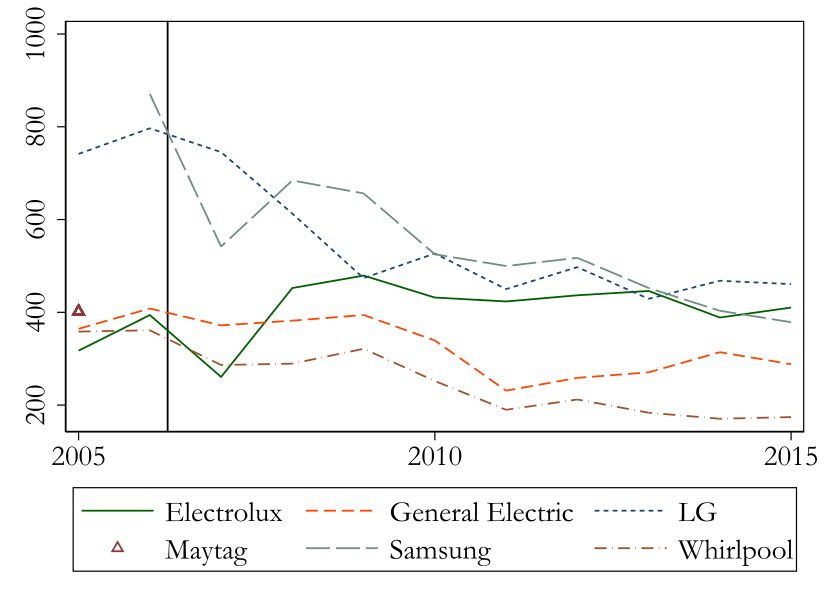
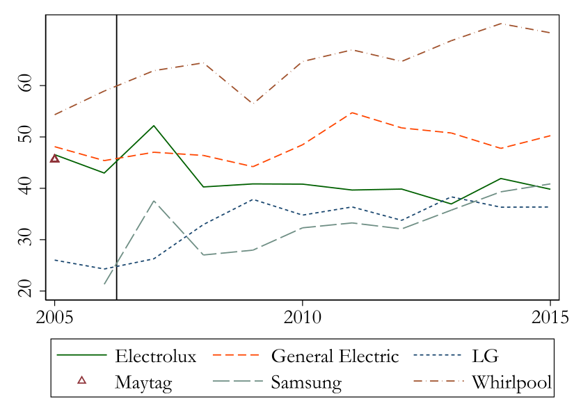
Notes: Marginal costs (left panel) and Lerner index (right panel) by brand owner over time. The vertical line indicates Whirlpool’s Maytag acquisition. Whirlpool includes Maytag products from 2006 onward.
| Marginal costs (2012 $) | |
|---|---|
| Real Exchange Rate | 186.087\(^{***}\) |
| (36.280) | |
| Distance (’000 km) | 8.544 |
| (8.275) | |
| Front Loader | 16.489 |
| (20.051) | |
| Agitator | -244.454\(^{***}\) |
| (26.785) | |
| Characteristics | Yes |
| Retailer FE | Yes |
| Brand FE | Yes |
| Brand time trends | Yes |
| Year FE | Yes |
| N | 1,586 |
Notes: The table presents regression results of product-level marginal costs on proxies for labor and shipping costs, product characteristics, fixed effects, and brand-specific time trends.
Table 5 quantifies how marginal costs depend on labor costs (captured by the deflated RER), shipping distance, product characteristics, and firm-specific fixed effects.
Although the estimate for distance-related transportation costs is noisy, the point estimate aligns closely with external reports. Specifically, shipping washers from Germany to the U.S. increases costs by approximately $59 (in 2012 dollars), matching Whirlpool’s reported cost in 2005.Whirlpool reports that shipping front-loaders from its plant in Germany to the U.S. cost $50 in 2005 ($57 in 2012 dollars). See https://www.nytimes.com/2005/06/17/business/worldbusiness/globalization-its-not-just-wages.html.
The deflated RER captures cross-country wage differences. For 2006, the RER was \(0.28\) for China, \(0.64\) for Mexico, and \(1\) for the U.S. (since it is normalized by U.S. prices).Within-country plant-level wage differences are arguably second-order compared to cross-country differences. Consequently, moving production from the U.S. to Mexico reduces labor costs by $67 per washer, while shifting to China reduces them by $134. However, relocating production to China raises transportation costs by $81. Thus, the total marginal cost impact of moving production from the U.S. to China or Mexico in 2006 would have been roughly equivalent.
Fixed cost bounds
Finally, Table 6 reports the estimated brand-level fixed cost bounds for offering a product. Recall that a product is defined as a combination of brand, retailer, and major washer characteristics. Hence, the estimated fixed cost intervals represent the costs associated with offering a specific product category (brand–characteristic combination) at a given retailer.
| Brand owner | Brand | 95% confidence sets | \(\mathbf{n^b}\) | |
|---|---|---|---|---|
| Maytag | Admiral | \(\left[ 6.3 , 12.6 \right]\) | 10 | |
| Amana | \(\left[ 1.7 , 5.1 \right]\) | 15 | ||
| Maytag | \(\left[ 5.3 , 25.3 \right]\) | 30 | ||
| Whirlpool | KitchenAid | \(\left[ 0.9 , 3.4 \right]\) | 10 | |
| Roper | \(\left[ 1.7 , 11.2 \right]\) | 20 | ||
| Whirlpool | \(\left[ 14.6 , 30.9 \right]\) | 30 | ||
| General Electric | General Electric | \(\left[ 2.5 , 18.4 \right]\) | 30 | |
| Hotpoint | \(\left[ 0.7 , 2.4 \right]\) | 15 | ||
| Electrolux | Frigidaire | \(\left[ 2.7 , 11.8 \right]\) | 20 | |
| Westinghouse | \(\left[ 0.6 , 2.1 \right]\) | 20 | ||
| LG | LG | \(\left[ 5.1 , 16.4 \right]\) | 20 | |
| Samsung | Samsung | \(\left[ 1.0 , 6.5 \right]\) | 10 | |
Notes: Brand-level fixed cost bounds are estimated from all active and potential products in 2005 and 2007.
The 95 percent confidence sets indicate that fixed costs tend to be larger for brands with higher market shares, such as Maytag and Whirlpool, compared to brands with lower market shares, such as KitchenAid, Hotpoint, and Westinghouse. This pattern could reflect that brands with larger market share require retailers to stock comprehensive product assortments, demanding greater floor space and higher marketing expenditures.
Welfare Effects of the Whirlpool Acquisition
With the estimated demand and supply parameters, I compare the welfare effects of alternative acquisitions of Maytag. First, I contrast the Whirlpool acquisition with a scenario in which Maytag remains independent, explicitly modeling endogenous product portfolios and employment outcomes. Although maintaining a standalone Maytag was not feasible, this scenario provides a useful intermediate step for the comparison between acquirers.
Second, I compare Whirlpool’s acquisition of Maytag to the hypothetical acquisition by Haier. The richest comparison incorporates how production relocations affect marginal costs, prices, consumer welfare, and employment.
Portfolio choice algorithm
Before presenting the welfare comparisons, I briefly discuss how firms endogenously choose product portfolios. Producers with market shares above 3 percent in any year can adjust portfolios (Electrolux, General Electric, LG, Maytag, Samsung, and Whirlpool).Smaller competitors’ portfolios, and products sold at retailers other than the major five, remain fixed. This leaves 135 potential products, alongside 69 products offered exogenously.
A known complexity in product portfolio choice games is equilibrium multiplicity. One way to identify the set of potential equilibria is to estimate the expected variable profits for all possible product entry combinations and then check whether there are any combinations of product entry costs contained in the fixed cost confidence sets that make these product portfolios an SPNE of the entry game.This is the approach taken by Eizenberg (2014) in a setting where there are four brands and four product types. After adding some additional restrictions, he ends up with \(2^9 = 512\) candidate equilibria. In my case, this is computationally infeasible since there are \(2^{135}\) candidate equilibria. Instead, following Fan and Yang (2020), I construct a heuristic portfolio optimization algorithm leveraging the observed pre-merger equilibrium as a starting point. This choice assumes that post-merger equilibria closer to pre-merger portfolios are more likely.
Specifically, firms iteratively optimize product portfolios by checking for profitable one-step deviations—either adding an inactive product or removing an active one—until no further profitable deviations exist. To reduce computational complexity, the algorithm optimizes portfolios at the brand rather than firm level. Because fixed costs are only set-identified, I repeat this process for 50 fixed-cost draws and report 95-percent confidence sets for welfare outcomes.Further technical details are in Appendix 14.1. Appendix Tables [app tab: cf merger fc 25] and [app tab: cf merger fc 75] present results for alternative fixed-cost draws.
The Whirlpool acquisition of Maytag
I first compare the Whirlpool acquisition to a scenario in which Maytag continues as a standalone firm, abstracting initially from production relocations. This intermediate step also corresponds to comparing acquisitions by Whirlpool and Haier in the product market if marginal costs remain unchanged, as Haier had no pre-merger U.S. presence.
The simulations rely on estimated demand and supply parameters from 2005–2015, assuming time-invariant preferences for characteristics. Brand-specific time trends and year fixed effects allow for time-varying preferences for brands and differences in outside options and input costs, respectively.
In scenarios without portfolio adjustments I hold firms’ 2005 product portfolios fixed, setting brand trends, deflated RER, and year fixed effects to 2005 levels. In scenarios with endogenous portfolios, I fix market conditions at their 2007 values, using all potential products from both 2005 and 2007.If product versions differ across years, I use the 2007 version. Since I observe the acquisition scenario associated with the greatest increase in market power, I observe conditions under which rivals like LG or Samsung had the strongest incentive to expand their product offerings, since less intensive competition encourages rival product entry. Thus, any product not offered by rivals post-merger would also likely have remained inactive absent the merger.
Table 7 shows that without portfolio adjustments, a Whirlpool acquisition raises average prices by 3.2 percent, increases Maytag and Whirlpool prices by 6.9 and 5.9 percent, respectively, and reduces consumer welfare by $167 million annually. Without relocations, the merger costs 127 domestic jobs due to reduced output and substitution toward imports. Including observed relocations post-merger, the Whirlpool acquisition reduces employment by 735 jobs, reflecting both variable labor (286 jobs shifting to Mexico) and fixed overhead employment (322 jobs from closing two Maytag plants).
| Product portfolios: | Pre-acquisition | Endogenous |
|---|---|---|
| Number of products | ||
| Maytag | – | -1.5 |
| – | [-3.5, 0.5] | |
| Whirlpool | – | -1.6 |
| – | [-3.3, 0.2] | |
| LG + Samsung | – | 0.4 |
| – | [-0.9, 1.8] | |
| Electrolux + GE | – | 1.3 |
| – | [-0.7, 3.3] | |
| Overall industry | – | -1.3 |
| – | [-4.2, 1.6] | |
| Prices and consumer welfare | ||
| Average price | 3.2% | 4.1% |
| [1.9%, 4.6%] | [3.5%, 4.7%] | |
| Maytag prices | 6.9% | 7.2% |
| [5.1%, 8.7%] | [5.4%, 8.9%] | |
| Whirlpool prices | 5.9% | 6.3% |
| [3.9%, 7.8%] | [3.0%, 9.6%] | |
| Consumer welfare | $-167M | $-224M |
| [$-215M, $-119M] | [$-267M, $-182M] | |
| Employment | ||
| Domestic jobs (w/o Maytag relocation) | -127 | -247 |
| [-175, -79] | [-411, -82] | |
| Domestic jobs (with Maytag relocation) | -735 | -1009 |
| [-869, -601] | [-1188, -829] |
Notes: Ninety-five percent confidence intervals for the first column are computed from 200 residual bootstrap draws. Confidence sets for the second column are based on 50 fixed cost draws for each potential product.
When firms adjust product portfolios endogenously, the merged entity reduces its product offerings to avoid cannibalization. However, the merger does not substantially alter rivals’ incentives to expand product lines relative to the standalone scenario.
Contrary to the Department of Justice’s assessment, endogenous portfolio adjustments exacerbate consumer harm, as fewer products remain available without significant portfolio expansions from rivals. These findings align with those of Fan and Yang (2020) and Fan and Yang (2025), contrasting with Wollmann (2018).
Notably, endogenous product choices also significantly amplify domestic employment losses, increasing them by 37 percent compared to fixed portfolios. Thus, considering portfolio decisions is crucial for accurately assessing employment impacts, even if policymakers focus primarily on labor outcomes.
Whirlpool vs. Haier as acquirers for Maytag
Next, I compare Maytag’s acquisition by Whirlpool versus Haier. Given Haier’s minimal pre-merger presence in the U.S. market, absent marginal cost changes, a Haier acquisition is equivalent for consumers to Maytag remaining standalone. Employment effects, however, differ substantially due to distinct production relocation strategies. I assume Haier would offshore all production to China, whereas Whirlpool’s observed post-merger plan offshored front-loader production to Mexico and maintained top-loader production domestically.
Table [tab: cf hai vs wp main] shows the differences between these two scenarios. Without marginal cost changes, the varying production locations have no consumer impact but significantly affect employment. Holding pre-merger product portfolios fixed, a Whirlpool acquisition preserves 566 more domestic jobs than a Haier acquisition. Combining this result with Table 7 illustrates the relative magnitude of employment impacts clearly: with unchanged Maytag production locations, Whirlpool’s acquisition results in a net loss of 127 U.S. jobs due to reduced output and substitution to foreign-produced competitor products. Allowing Whirlpool’s observed production relocations increases this loss to 735 jobs. Conversely, allowing Haier’s production adjustments reverses the sign, making Whirlpool’s acquisition preferable for domestic employment by 566 jobs. Balancing this against the consumer welfare loss from Whirlpool’s acquisition implies each preserved job must be valued at $293,000 per year to offset consumer harm (considering only U.S. consumer welfare and employment), or $150,000 when also accounting for industry profits.
lccccc & & &
Cost adjustments: & None & Offshoring & & None
& Offshoring
Cost pass-through & & & & &
& – & 86% & & – & 85%
& – & [76%, 96%] & & – & [84%, 87%]
& – & 85% & & – & 84%
& – & [72%, 98%] & & – & [83%, 85%]
Prices and consumer welfare & & & &
&
& 3.2% & 4.6% & & 4.1% & 5.5%
& [1.9%, 4.5%] & [2.0%, 7.3%] & & [3.5%, 4.7%] &
[4.7%, 6.2%]
& $-166M & $-215M & & $-222M & $-271M
& [$-213M, $-119M] & [$-296M, $-133M] & & [$-264M,
$-179M] & [$-316M, $-225M]
Employment & & & & &
& 566 & 571 & & 754 & 797
& [400, 733] & [407, 734] & & [559, 949] & [612,
982]
Industry profits & & & & &
& $81M & $55M & & $79M & $47M
& [$58M, $104M] & [$2M, $107M] & & [$54M, $105M] &
[$19M, $74M]
& $81M & $55M & & $106M & $83M
& [$58M, $104M] & [$2M, $107M] & & [$80M, $132M] &
[$56M, $111M]
Maytag + Whirlpool profits & & & &
&
& – & 5.9% & & – & 4.7%
& – & [-4.3%, 16.0%] & & – & [3.9%, 5.5%]
& $23M & $-16M & & $4M & $-38M
& [$5M, $41M] & [$-82M, $51M] & & [$-37M, $44M] &
[$-81M, $6M]
& $23M & $-16M & & $40M & $11M
& [$5M, $41M] & [$-82M, $51M] & & [$24M, $57M] &
[$-5M, $26M]
& & & &
& $293k & $376k & & $299k & $344k
& [$209k, $377k] & [$229k, $524k] & & [$203k, $396k]
& [$250k, $438k]
& $150k & $280k & & $157k & $238k
& [$90k, $211k] & [$59k, $502k] & & [$100k, $213k] &
[$172k, $304k]
Notes: The first two columns compare the effect of a Maytag acquisition by Whirlpool with that of one by Haier without product portfolio adjustments. The final two columns account for endogenous portfolio adjustments. Columns (1) and (3) do not allow for acquisition-related cost changes. Columns (2) and (4) account for labor and shipping cost changes due to offshoring. Ninety-five percent confidence intervals for the first two columns are computed from 200 residual bootstrap draws. Confidence sets for final two columns are based on 50 fixed cost draws for each potential product.
Finally, I allow marginal costs to adjust based on production relocations, incorporating estimated labor and shipping costs from Table 5.Given the imprecise distance coefficient estimation in Table 5, I fix it at its point estimate across bootstrap draws. Appendix Table [app tab: wf wp vs. hai gamma bootstrapped] relaxes this constraint, yielding wider confidence intervals for offshoring-related estimates without affecting the main conclusions. Without product portfolio adjustments, Whirlpool passes through 86 percent of marginal cost savings to consumers, while Haier passes through 85 percent. Importantly, although Whirlpool almost fully passes on the cost savings for relocated Maytag products, it simultaneously raises prices on unaffected Whirlpool products, reducing overall consumer gains. The pass-through rate therefore overstates the consumer benefits of cost savings after a Whirlpool acquisition.
Although relocating production from the U.S. to Mexico or China yields similar cost savings, Haier’s complete offshoring to China results in an additional 6 percent marginal cost reduction across Maytag products relative to Whirlpool’s partial offshoring, which maintains top-loader production in the United States. This widens the consumer welfare gap between the two scenarios.Direct comparison in Table [tab: cf hai vs wp main] isolates only relative differences. For total effects of offshoring, see Appendix Tables [app tab: wp vs. none] and [app tab: hai vs. none], comparing each acquisition scenario against no acquisition.
Additionally, cost reductions from offshoring slightly reduce U.S. jobs further—by 24 under Whirlpool and by 29 under Haier. When fully accounting for marginal cost changes, each preserved job under Whirlpool must now be valued at $376,000 annually to offset consumer harm (consumer welfare and jobs only), or $280,000 with industry profits.
With endogenous portfolio adjustments and offshoring cost changes, the difference in U.S. manufacturing jobs increases to 797. To offset consumer harm, each protected job needs to be worth at least $344,000 per year.
Depending on the assumptions made, the point estimates for the necessary job value to offset consumer harm range from $150,000 to $376,000 per year. However, these figures alone are insufficient to assess whether employment effects plausibly offset product market harm. Ideally, I would measure the full value of these jobs to local labor markets. Section 3 suggests these jobs are valuable, though average wages alone likely underestimate their value due to multiplier effects. To contextualize the estimates, I turn to prior studies on the local labor market value of multinational jobs and those assessing job values necessary to offset consumer losses from trade policies.
Setzler and Tintelnot (2021) find that each additional foreign multinational job increases the local labor market’s total wage bill by $113,000 annually through direct and indirect local labor market effects. The literature on earnings losses of displaced workers after mass layoffs suggests that such earnings losses are persistent. For instance, Jacobson et al. (1993) find earnings losses of 40 percent in the short-term and 25 percent in the long-term using data from Pennsylvania in the 1970s and 1980s. Couch and Placzek (2010) reproduce this analysis for Connecticut (1993–2004) and find earnings losses of 32 percent short-term and 15 percent long-term. Similarly, Schmieder et al. (2023) document long-term earnings losses of about 15 percent lasting at least 15 years following mass layoffs in Germany.
Alternatively, prior work evaluating U.S. sector-specific tariffs also provides valuable benchmarks. Hufbauer and Lowry (2012) estimate each job preserved by the 2011 safeguard tariffs on tire imports from China would need to be worth at least $900,000 annually to offset consumer losses, while Flaaen et al. (2020) calculate that jobs created from the 2018 washing machine safeguard tariffs would need to be worth at least $817,000 per year.
Beyond wages, local job availability generates additional benefits, suggesting that the increase in the local wage bill from Setzler and Tintelnot (2021) is likely a lower bound for the full value of an appliance manufacturing job to the U.S. economy. Although this figure falls at the lower end of my estimated range, the magnitudes are comparable, indicating that domestic employment benefits from the Whirlpool acquisition are economically meaningful relative to consumer welfare losses.
Thus far, the analysis considered overall consumer and worker impacts. Yet, the distributional implications of the alternative acquisitions are also significant. While an additional thousand manufacturing jobs may not affect national employment or wages appreciably, Section 3 shows local impacts are substantial and persistent. Figure 1 highlights that washer manufacturing jobs are geographically concentrated in a small number of counties in Illinois, Iowa, Michigan, Ohio, and South Carolina.
Therefore, consumer harm from the merger is broadly dispersed nationwide, whereas employment benefits are highly concentrated geographically. If households exhibit diminishing marginal utility of income and job losses predominantly affect less affluent regions, a Whirlpool acquisition could yield a higher aggregate welfare (sum of domestic worker and consumer welfare) despite consumer welfare losses exceeding the wage gains. Additionally, accounting for nonwage outcomes related to employment—such as mental and physical health—further supports the case that Whirlpool’s acquisition may offer superior overall domestic welfare relative to Haier’s.
Conclusion
This paper provides a framework to quantify the trade-off that policy choices can generate between consumers and workers. To capture the incentives firms have to adjust their product portfolios in response to policy changes, I explicitly model endogenous portfolio decisions. To evaluate employment effects, I model the relationship between the product market equilibrium and labor demand. I find that incorporating product market responses is key to estimating employment effects.
I apply this framework empirically to analyze how foreign competition influences the consumer welfare and domestic employment effects of mergers. Specifically, I examine Whirlpool’s acquisition of Maytag and compare its impacts to a hypothetical acquisition by Haier. I find that the Whirlpool acquisition significantly harmed consumers and that rivals had limited incentives to expand their product offerings. However, while an alternative Haier acquisition would have mitigated consumer harm, it would also have substantially increased domestic job losses. Finally, I calculate the necessary value of a domestic job to offset these consumer welfare losses, quantifying the trade-off explicitly.
The preceding analysis should not be viewed as an endorsement of allowing anticompetitive mergers to preserve domestic jobs. Such mergers still harm consumers (and foreign workers) and may hinder the efficient long-run reallocation of resources. Rather, the methodology developed here can help policymakers identify and evaluate mergers where employment impacts are particularly significant. Procompetitive merger enforcement could then be complemented by targeted labor market policies, such as the Trade Adjustment Assistance Program (see (Hyman et al. 2023)). Such an integrated approach could reconcile the interests of workers and consumers, making rigorous merger enforcement politically more viable.